
|
|
|
| Contact Us | Visit Us | UCAR People Search | Numerics| Assimilation| Turbulence| Statistics |

For all of these examples you should load the fields package and also the datasets. (You only need to do this once when starting R.) Fields is available as a contributed package in the Comprehensive R Archive Network CRAN
library(fields)
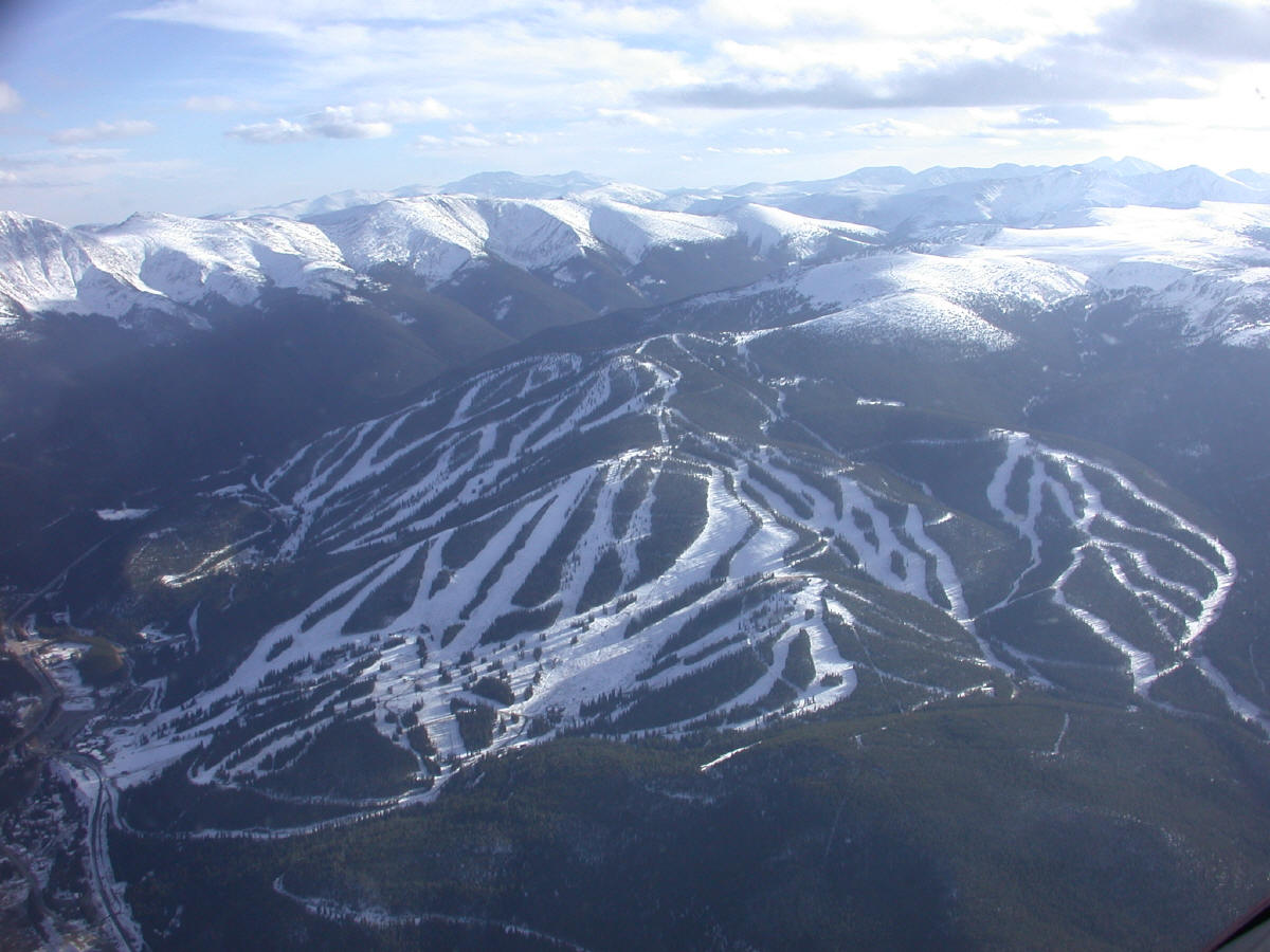
attach("RData.riflesight.bin")
Note that the perspective and image plots actually use the lon lat coordinates. But the Euclidean transformation is used for surface fitting and estimating derivatives.
# find spacing in meters of the lon and lat grid.
# and scale of longitude coordinates to give equal distance
# Because this region is so small we will ignore the curvature of
# coordinates on sphere.

dlat<- RifleDEM$y[2]- RifleDEM$y[1]

dx<- rdist.earth( cbind( RifleDEM$x[1:2],  RifleDEM$y[c(1,1)] ),
  miles=FALSE)[2,1] *1000
dy<- rdist.earth( cbind( RifleDEM$x[c(1,1)],  RifleDEM$y[1:2] ) ,
   miles=FALSE)[2,1] *1000

dlon<- RifleDEM$x[2]- RifleDEM$x[1]
dlat<- RifleDEM$y[2]- RifleDEM$y[1]

# Create all the grid locations explicitly
# converting  to a approximate cartesian grid in meters

make.surface.grid( list( x=(RifleDEM$x- RifleDEM$x[1])*dx/dlon,
                         y= (RifleDEM$y- RifleDEM$y[1])*dy/dlat) )-> Rgrid

# Rtrial is the ski run in the meter Euclidean coordinates.
Rtrail<- cbind(
 (rifle.trail[,1] - RifleDEM$x[1])*dx/dlon,
 (rifle.trail[,2] - RifleDEM$y[1])*dy/dlat )

# to find slopes need to parameterthe 1-d curve of the ski run
# by arc length
 N<- nrow( rifle.trail)
 rD<- sqrt(diff( Rtrail[,1])**2 + diff( Rtrail[,2])**2)
 trail.D<- c(0,cumsum( rD))
#First remove spatial linear drift by least squares fit before finding
# the variogram.
zR<- lsfit( Rgrid, c( RifleDEM$z))$residuals
zR<- matrix( zR, ncol= ncol( RifleDEM$z), nrow= nrow( RifleDEM$z))
# see help(vgram.matrix) for details on this function
# R is set to look at all pairs within a distance of about 6.5 grid spacings
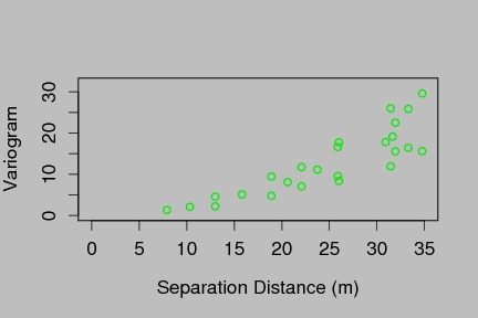
vgram.matrix( zR, R= 65, dx=dx, dy=dy) -> look
# A nice plot converting distance in scaled lon/lat to meters.
fields.style()
plot( look$d.full, look$vgram.full, xlab="Separation Distance (m)",
ylab="Variogram", xlim=c(0, 35),ylim=c(0,32), col=2)
# Kriging with compactly supported Wendland covariance function
# The range (theta) controls support.

theta<- 30
lambda<-0

mKrig( Rgrid, c( RifleDEM$z), cov.function="wendland.cov", k=2,
             theta=theta,
             lambda=lambda,mean.neighbor=50 )-> rifle.fit

rifle.trail.elev<- predict(rifle.fit, Rtrail)
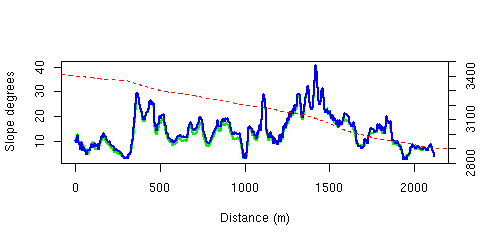
# computing slope based on 1-d space curveIt can be checked that the two estimates of slope are very similar.
# and interpolating cubic spline
trail.slope<- splint( trail.D,rifle.trail.elev, trail.D, derivative=1)
trail.degrees<- - atan( trail.slope)*(360/(2*pi))
# The correct way to find by slope taking partials of elevation surface
#
rifle.trail.der<- predict(rifle.fit, Rtrail,derivative=1)
# First find unit tangent vector along run
#
xp<- splint( trail.D,rifle.trail[,1], trail.D, derivative=1)
yp<- splint( trail.D,rifle.trail[,2], trail.D, derivative=1)
R<- sqrt( xp**2 + yp**2)
xp<- xp/R
yp<- yp/R
# find directional derivative based on tangent vector
trail.slope2<- xp*rifle.trail.der[,1] + yp*rifle.trail.der[,2]
trail.degrees2<- - atan( trail.slope2)*(360/(2*pi))
  matplot( trail.D, cbind(trail.degrees,trail.degrees2),
                      type="l", xlab="Distance (m)",
              ylab="Slope degrees",lwd=2, col=c(2,3),lty=1 )

# Just for fun ... add in elevation drop
  par( usr=c(0,2000,2800,3500) )
  lines( trail.D, rifle.trail.elev,type="l", xlab="Distance (m)",
                ylab="Elevation (m)",col=4, lwd=1.5, lty=2)
  axis( 4)
The data sets, software and related content in and linked to these pages are intended for scientific and mathematical research. The authors do not guarantee the correctness of the data, software or companion text. Please see the UCAR Terms of Use listed below.
© 2010, UCAR |
Privacy Policy |
Terms of Use |
Contact UCAR | Visit UCAR |
Sponsored by
