Description: US precipitation and temperature data 1895-1997

This is a nearly complete record in R binary format for the monthly weather station data for the continential US from 1895 through 1997. Variables are the monthly average daily minimum temperature, average daily maximum temperature and total precipitation. Temperature units are degree C and precipitation is in millimeters.

The R binary data file RData.USMonthlyMet.bin can be obtained from the directory http://www.image.ucar.edu/public/Data and is 28.2Mb in size. The R script make.RData.USMet.R was used to create these objects from the full data sets that include infilled values. e (244kb) text file USmonthly.names.txt is a table ( station code, place name) that can be used to find the geographic name of a station. Not all the precipitation stations are in this list however.

Accessing in R

In R, the command line:

attach("RData.USMonthlyMet.bin")

will attach these data objects to your current session. Use the R function load to add these objects permanently to your R workspace.

Format:

The individual data objects in components are two tables of the meta information concerning station locations (UStinfo, USpinfo) and three, 3-dimensional arrays of the actual monthly statistics (UStmax,UStmin, USppt). Note that the temperature and preciptiation stations may differ and that is the reason for two separate "info" objects.

UStinfo, USpinfo

Are each data frames with components

• station.id A six character string that is the unique station code. First two digits indicate the station's state. e.g. 01XXXX == Alabama
• elev Elevation in meters
• lon Longitude in degrees
• lat Latitude in degrees
• station.names 12 character station name

UStmin, UStmax

Are each dimensional arrays 103X12X8125 indexing year, month and station.
Units are in degrees centigrade and years are from 1895 through 1997.

USppt

A three dimensional array 103X12X11918 indexing year, month and station.
Units are in total millimeters of precipitation during the month and years are from 1895 through 1997.

Source

The data is a compendium of different levels of weather data ranging from stations taking regular hourly measurements, such as those at airports, to cooperative observer stations where the records may only include daily values, have gaps in time or might not measure both temperature and precipitation. The original source for the data are the data archives at the National Climatic Data Center (http://www.ncdc.noaa.gov) although these data have been further processesd to combine stations at similar locations and eliminate stations with short records. These data formed the basis for the 103-Year High-Resolution Precipitation Climate Data Set for the Conterminous United States ftp://ftp.ncdc.noaa.gov/pub/data/prism100 this is an interpolation of the observational data to a 4km grid that takes in account and topography.

Examples

Load the big data set and also fields library

attach("RData.USMonthlyMet.bin")
library(fields)

Some desriptive plots of station density

# descriptive plots
png("fig1.png",width=480, height=360)
plot( UStinfo[,3:4], col="red", pch=".", cex=2, xlab="", ylab="",
axes=FALSE)
US(add=TRUE, col=" blue")
title("Temperature stations 1895-1997", cex=2)
dev.off()

png("fig2.png",width=480, height=360)

temp1<- apply(  is.na((UStmax+UStmin)[,7,]) , 1, "sum")
temp1<- 8125- temp1

temp2<- apply( is.na( (UStmax+UStmin)[,1,]) , 1, "sum")
temp2<- 8125- temp2

ppt1<- apply( is.na( (USppt)[,7,]) , 1, "sum")
ppt1<- 11918- ppt1

ppt2<- apply( is.na( (USppt)[,1,]) , 1, "sum")
ppt2<- 11918- ppt2

matplot( 1895:1997, cbind( temp1,  ppt1, temp2,ppt2), type="l", 
 lty=c( 1,1,2,2),
   col=c("red", "blue"), xlab="year", ylab="number of stations",
lwd=1.5, cex=2)

title("Number of reporting stations for 
July (solid) and Jan (dashed) 
precipitation (blue), temperature (red)")
dev.off()

Some summary plots of the Colorado subset

Creating summer monthly temperature subset for Colorado.

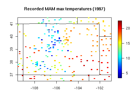
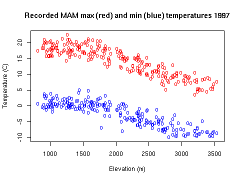
ind<- (UStinfo$lon < -101) &  (UStinfo$lon> -109.5)
ind<- ind & (UStinfo$lat<41.5) &  (UStinfo$lat>36.5)

# (3 4 5) (6 7 8) (9 10 11)  (12 1 2)
CO.tmax.JJA<- apply( UStmax[,6:8,ind],c(1,3), "mean")
CO.tmin.JJA<- apply( UStmin[,6:8,ind],c(1,3), "mean")

CO.loc<- UStinfo[ind,3:4]
CO.elev<- UStinfo$elev[ind]
CO.id<- UStinfo$station.id[ind]

Plot of 1997 summer maximum temperatures and the 30 year average temperatures against elevation.

png("fig3.png",width=480, height=360)
quilt.plot( CO.loc,CO.tmax.JJA[103,]  )
US( add=T)
title( "Recorded JJA mean daily max temperatures (1997)")
dev.off()

png("fig4.png",width=480, height=360)
ind<- (1990:1961) - 1894
temp1<- apply( CO.tmin.JJA[ind,],2,"mean", na.rm=TRUE)
temp2<- apply( CO.tmax.JJA[ind,],2,"mean", na.rm=TRUE)

matplot( CO.elev, cbind( temp1,temp2),
  pch=".", type="p",
  col=c("red", "blue"), 
  xlab="elevation (m)", ylab="Temperature (C)", cex=2)
title( " JJA mean daily max/min temperatures (1961-1990))", cex=2)
dev.off()

---

DISCLAIMER:

The data sets, software and related content in and linked to these pages are intended for scientific and mathematical research. The authors do not guarantee the correctness of the data, software or companion text. Please see the UCAR Terms of Use listed below.