Estimating Spatial Covariance Parameters in Precipitation Anomalies Using Covariance Tapering

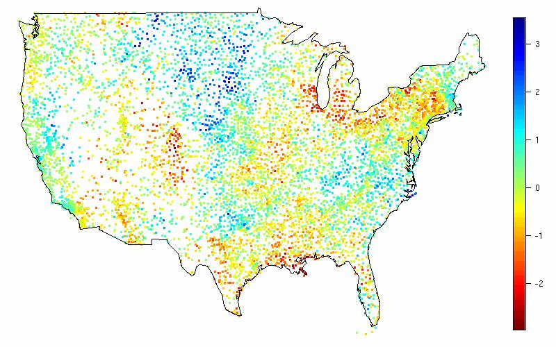
This example illustrates the use of covariance tapering in estimating the spatial covariance parameters of a large dataset. The motivation behind this approach and further details can be found in "Covariance Tapering for Likelihood Based Estimation in Large Spatial Datasets" by Kaufman, Schervish, and Nychka (2007). The data are yearly precipitation anomalies from 1962 at US weather stations. This means they are standardized with respect to the long run mean and standard deviation of each station.

The files for the example are contained in taperexample.zip. The data file is anom1962.RData. This contains a matrix loc of the station locations (latitude and longitude), and a vector of anomalies z.

You will need several R packages to run the example: fields, spam, maps, and xtable. These are all available from CRAN.

The R files assume you will be running them in order. Each one will store its results in a .RData file of the same name. They are:

1. likcalc.R - calculate the profile negative log likelihoods (standard and tapered) over a grid
2. maxlik.R - minimize the profile negative log likelihoods, using the values from likcalc.R to guide ranges for maximization
3. infcalc.R - calculate the information matrices and create confidence intervals
4. timing.R - carry out detailed timing of a single function evaluation

You can also make a map of the observations like the one above by using plotdata.R.

DISCLAIMER:

The data sets, software and related content in and linked to these pages are intended for scientific and mathematical research. The authors do not guarantee the correctness of the data, software or companion text. Please see the UCAR Terms of Use listed below.

UCAR : NCAR : CISL : IMAGe : [  CMG   DAReS   GSP   RISC   TNT  ]
For problems with the page, contact Tim Hoar - thoar 'at' ucar 'dot' edu

© 2010, UCAR | Privacy Policy | Terms of Use | Contact UCAR | Visit UCAR | Sponsored by