Maximum 8-hr Daily Average Ground-level Ozone

Download the file, ozmax8.dat, which has the actual ozone measurements (max 8-hr daily average). Units are concentrations in parts per billion (PPB). Also, download the file, ozmax8.info.q, This is a list with information about the data set: station.no, lat, lon, dates. The times are in julian days where day 1 = JAN-01-1960. The actual times start on April 1, 1995. The ozone "season" runs from April through October ( 184 days) over five years (1995 - 1999). Alternatively, if only data from the North Carolina subset is desired, download the file NCdat.R, which has the daily maximum 8-hr average ozone data (ozmax8), the locations for the N.C. subset (loc) and the time points (dates). The standardized data for this subset are also available (NCstdO3.dat).

Load into R

From an R session, use the following commands to load them into R:

 ozmax8 <- matrix( scan("ozmax8.dat"), 920,513) 
 source("ozmax8.info.q") 
# names( ozmax8.info) 
# are "stat.no" "lat"     "lon"     "dates"   "loc" 
#
# to plot station locations
plot( ozmax8.info$lat, ozmax8.info$lon)


# time series plot of first station
plot(  ozmax8.info$date, ozmax8[,1])
#
#
# the next example requires the fields package from CRAN
#
 library( fields)
 corr <- cor( ozmax8, use = "pairwise")
 up <- col( corr) > row( corr) 
 corr <- corr[ up] 
 dist <- rdist.earth( ozmax8.info$loc)[up] 
 plot( dist, corr, type="n", xlab="distance (miles)", ylab="cor") 
 points( dist, corr, pch=".", col="blue") 
 bplot.xy( dist, corr, add=TRUE) 
 rm( corr, dist, up) 

# Working with the dates
# Sorry yet another R package. I find much of the date stuff 
# incomprehensible!

library( chron)
# to extract calendar information
start<- c(month = 1, day = 1, year = 1960)
month.day.year( ozmax8.info$dates, origin.= start)-> look

# look has components of month, day, year

# to find the "day of year" necessary to model an annual cycle

# first reset so that day 1 of the cycle is  Jan 1. 
day.of.year<- (ozmax8.info$dates- julian( 12,31,1994, origin.=start))
day.of.year<- day.of.year%%365.25

The result should look like the plot below.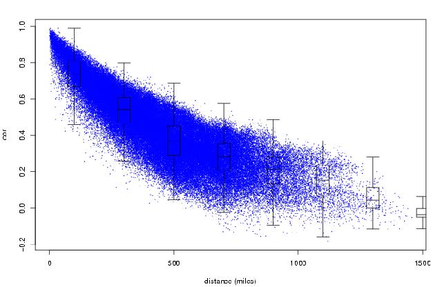

UCAR : NCAR : CISL : IMAGe : [  CMG   DAReS   GSP   RISC   TNT  ]
For problems with the page, contact Tim Hoar - thoar 'at' ucar 'dot' edu

© 2010, UCAR | Privacy Policy | Terms of Use | Contact UCAR | Visit UCAR | Sponsored by