Fields Demo/tutorial:
Some examples created by Doug Nychka using functions from the Fields software package designed to quickly familiarize users with some of the tools and methods available. For more organized coverage of this software, check out the Fields On-Line Manual.
Some color-coding makes the tutorial easier to follow, so here goes
(by convention, all comments are preceeded by a '#'):
# These are comments
These are commands to faciliate
"cutting&pasting", we omit the R prompt ('>')
These are output
Because we can, the graphics are included after the commands that generated
them.
Rats ...
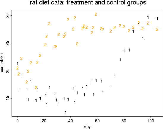
This was experiment that involved feeding one group of rats an appetite
supressant while the treatment was withheld from the contol group
(naturally). The treatment was removed around day 65. The food intake in
the control group is in rat.diet$con. The food intake for
the rat treatment group is rat.diet$trt.
plot( rat.diet$t, rat.diet$trt)
# complete experiment
matplot( rat.diet$t, cbind( rat.diet$trt, rat.diet$con),
ylab="food intake", xlab="day")
title(" rat diet data: treatment and control groups")
 # fit a nonparametric curve ( a cubic spline) to these data.
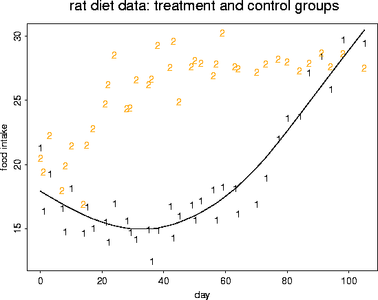
# curve has 4 degress of freedom
out <- sreg( rat.diet$t, rat.diet$trt, df=4)
out
Call:
sreg(x = rat.diet$t, y = rat.diet$trt, df = 4)
Number of Observations: 39
Effective degrees of freedom: 4
Residual degrees of freedom: 35
Residual root mean square: 1.433
Lambda ( smoothing parameter) 235.6
# take a look at the fit by adding a line to the current (active) figure
lines( rat.diet$t, out$fitted.values, col=1, lwd=2)
 # fit another spline (with 12 degrees of freedom)
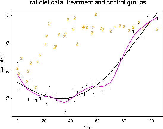
out <- sreg( rat.diet$t, rat.diet$trt, df=12)
out
Call:
sreg(x = rat.diet$t, y = rat.diet$trt, df = 12)
Number of Observations: 39
Effective degrees of freedom: 12
Residual degrees of freedom: 27
Residual root mean square: 1.14
Lambda ( smoothing parameter) 1.202
lines( rat.diet$t, out$fitted.values, col=4, lwd=2)
 # now fit the spline using GCV to choose the model degrees of freedom
out <- sreg( rat.diet$t, rat.diet$trt)
out
Call:
sreg(x = rat.diet$t, y = rat.diet$trt)
Number of Observations: 39
Effective degrees of freedom: 7.5
Residual degrees of freedom: 31.5
Residual root mean square: 1.247
Lambda ( smoothing parameter) 11.07
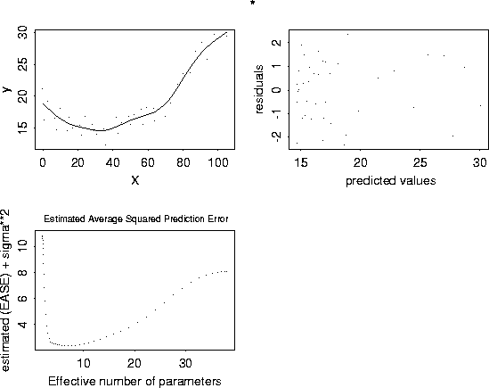
plot( out, pch="*")
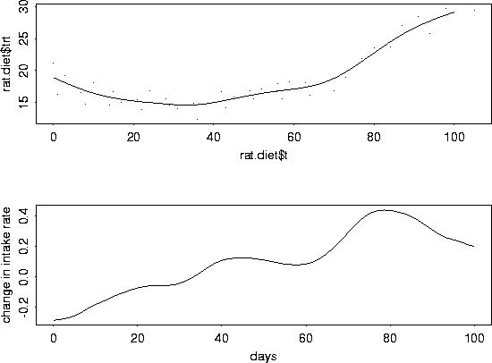
 # Plot GCV curve and its derivative by creating some temporary arrays.
# Note we can subdivide the plot window
x <- seq( 0, 100,, 80)
hold <- predict( out, x)
hold2 <- predict( out, x, derivative=1)
set.panel(2,1)
plot( rat.diet$t, rat.diet$trt)
lines( x, hold)
plot( x, hold2, xlab="days", ylab="change in intake rate", type="l")
 # To get some standard errors, it is easier to switch to the
# thin plate spline function ... Tps
out <- Tps( rat.diet$t, rat.diet$trt)
out
Call:
Tps(x = rat.diet$t, Y = rat.diet$trt, cov.function = "Thin plate spline radial
basis functions (rad.cov) ")
Number of Observations: 39
Degree of polynomial null space ( base model): 1
Number of parameters in the null space 2
Model degrees of freedom: 7.5
Residual degrees of freedom: 31.5
GCV estimate for sigma: 1.387
MLE for sigma: 1.356
lambda 0.00037
rho 4936
sigma^2 1.839
set.panel( 1,1)
fit <- predict( out, x)
se <- predict.se( out, x)
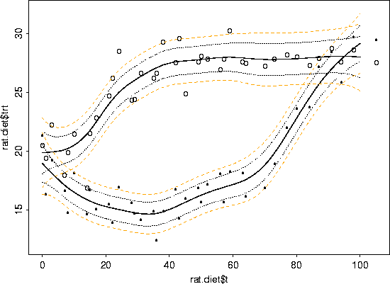
# plot data,
# GCV spline, and
# upper and lower pointwise CI's
plot( rat.diet$t, rat.diet$trt, ylim=c(12,32), pch="*")
lines( x, fit, lwd=2)
lower <- fit - 1.96* se
upper <- fit + 1.96*se
lines(x, lower, lty=2)
lines(x, upper, lty=2)
# Bonferoni bounds
bonf <- qnorm( .025/39)
blower <- fit - bonf* se
bupper <- fit + bonf*se
lines(x, blower, lty=3, col=2)
lines(x, bupper, lty=3, col=2)
# and now for the control group of rats.
# (same strategy as we used for the trial group of rats)
out <- Tps( rat.diet$t, rat.diet$con)
out
Call:
Tps(x = rat.diet$t, Y = rat.diet$con, cov.function = "Thin plate spline radial
basis functions (rad.cov) ")
Number of Observations: 39
Degree of polynomial null space ( base model): 1
Number of parameters in the null space 2
Model degrees of freedom: 7.6
Residual degrees of freedom: 31.4
GCV estimate for sigma: 1.579
MLE for sigma: 1.521
lambda 0.00034
rho 6769
sigma^2 2.314
fit <- predict( out, x)
se <- predict.se( out, x)
points( rat.diet$t, rat.diet$con, pch="o")
lines( x, fit, lwd=2)
lower <- fit - 1.96* se
upper <- fit + 1.96*se
lines(x, lower, lty=2)
lines(x, upper, lty=2)
bonf <- qnorm( .025/39)
blower <- fit - bonf* se
bupper <- fit + bonf*se
lines(x, blower, lty=3, col=2)
lines(x, bupper, lty=3, col=2)
 # what is a spline doing to the data?
out <- Tps( rat.diet$t, rat.diet$trt )
A <- make.Amatrix( out )
look <- A%*% rat.diet$trt
# predicted from the hat matrix times y
look2 <- predict( out )
# predicted from the Tps object
# list them out to compare
cbind( look,look2)
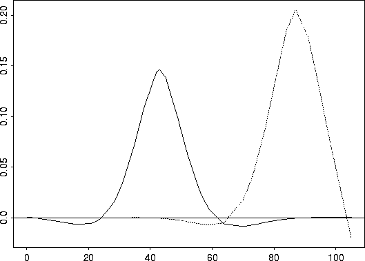
# the rows of A are the weights applied to the observed data to
# give the spline at the points
row20 <- c(A[20,])
row35 <- c( A[35,])
matplot( rat.diet$t , cbind( row20, row35), type="l", col=1)
yline( 0)
Ozone ...
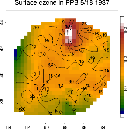
# lets load the ozone2 dataset and make a map # map of ozone data sites data(ozone2) names(ozone2) [1] "lon.lat" "y" "chicago.subset" US( xlim= c(-93.6,-82.8), ylim=c(36.7, 44.5) ) points( ozone2$lon.lat, pch="o")# take a look at day 16: June 18, 1987 # removing the missing values complicates things a bit, but not much. y16.full <- c(ozone2$y[16,]) good <- !is.na(y16.full) y16 <- y16.full[good] x <- ozone2$lon.lat[good,] # OK now we have removed the missing values for day 16 and we # called it "y16", their locations are in "x" # thin plate spline out <- Tps( x, y16 ) out Call: Tps(x = x, Y = y16, cov.function = "Thin plate spline radial basis functions (rad.cov) ") Number of Observations: 147 Degree of polynomial null space ( base model): 1 Number of parameters in the null space 3 Model degrees of freedom: 74.6 Residual degrees of freedom: 72.4 GCV estimate for sigma: 9.275 MLE for sigma: 8.392 lambda 0.00014 rho 489200 sigma^2 70.43 surface( out)
# try out some other spatial covariances # One example of a covariance function is the exponential: # exp.cov or exp.cov.S out <- Krig( x, y16, exp.cov, theta=2 ) surface(out)
# some more complicated plots look <- predict.surface( out ) image.plot(look, graphics.reset=F ) US( add=T )
# a better covariance set.panel() out <- Krig( x, y16, exp.earth.cov, theta=343) plot(out)
surface(out)
# find some time averaged fields ozone.cor <- COR( ozone2$y) mean.tps <- Tps( ozone2$lon.lat, ozone.cor$mean, return.matrices=F) sd.tps <- Tps( ozone2$lon.lat, ozone.cor$sd, return.matrices=F) # make up a data set of pairwise distance by correlation. upper <- col(ozone.cor$cor) > row(ozone.cor$cor) cgram.oz <- list( d=rdist.earth( ozone2$lon.lat)[upper], cor=ozone.cor$cor[upper]) # plot correlations as a function of distance plot( cgram.oz$d, cgram.oz$cor, xlab="correlation", ylab="distance",pch=".") title( "sample correlation as function of distance")
# this is where the 343 came from for the range parameter library(nls) cgram.fit <- nls( cor ~ alpha* exp( -d/theta), cgram.oz, start= list( alpha=.95, theta=200)) summary( cgram.fit) Formula: cor ~ alpha * exp(-d/theta) Parameters: Estimate Std.Error t value Pr(>|t|) alpha 9.306e-01 3.701e-03 251.5 <2e-16 *** theta 3.434e+02 2.403e+00 142.9 <2e-16 *** --- Signif. codes: 0 `***' 0.001 `**' 0.01 `*' 0.05 `.' 0.1 ` ' 1 Residual standard error: 0.1216 on 11626 degrees of freedom Correlation of Parameter Estimates: alpha theta -0.8384 # OK now we are going to fit the "right" model. # We standarize the ozone and fit a surface to the standardized data # (and undo things for predicting and inference) fit.GCV <- Krig( x, y16, cov.function=exp.earth.cov,theta=343, sd.obj=sd.tps, mean.obj= mean.tps, m=2) summary( fit.GCV) CALL: Krig(x = x, Y = y16, cov.function = exp.earth.cov, m = 2, mean.obj = mean.tps, sd.obj = sd.tps, theta = 343) Number of Observations: 147 Number of unique points: 147 Degree of polynomial null space ( base model): 1 Number of parameters in the null space 3 Effective degrees of freedom: 115.6 Residual degrees of freedom: 31.4 MLE sigma 0.2859 GCV est. sigma 0.3129 MLE rho 7.698 Scale used for covariance (rho) 7.698 Scale used for nugget (sigma^2) 0.08175 lambda (sigma2/rho) 0.01062 RESIDUAL SUMMARY: min 1st Q median 3rd Q max -0.593400 -0.075240 0.002854 0.079600 0.422300 COVARIANCE MODEL: exp.earth.cov A correlation model was fit: Y is standardized before spatial estimate is found DETAILS ON SMOOTHING PARAMETER: Method used: Cost: 1 lambda trA GCV GCV.one GCV.model shat 0.01062 115.63608 0.45895 0.45895 NA 0.31292 Summary of estimates for lambda lambda trA GCV shat GCV 0.01062 115.6 0.4590 0.3129 GCV.one 0.01062 115.6 0.4590 0.3129 # the finale look <- predict.surface( fit.GCV ) look2 <- predict.surface.se( fit.GCV ) set.panel() par( pty="s") image.plot( look, graphics.reset=F) contour( look2, add=T) title("Surface ozone in PPB 6/18 1987") dev.off()
