|
Table of Contents |
|
1. Introduction
2. Thin Plate Splines: Tps 3. Spatial Process Models: Krig 4. Simulating Random Fields (sim.rf) 5. Spatial Predictions for Large Data Sets
|
|
Printable version of Fields Manual
Back to Fields Home Page |
2.1 The Model
where f(X) is a d dimensional surface, and the object is to fit a thin plate spline surface to irregularly spaced data, e are random errors with zero mean, uncorrelated and with variances
 /W_i. A
mathematical summary of this type of spline is given in the last section of this
manual.
2.2 Cross-Validation
 , a parameter
controlling the amount of smoothing. For the case of one dimension and
m = 2, the estimate reduces to the usual cubic
spline.
 , varies from zero
to infinity. When
  = 0 the spline estimate
interpolates the data and has a residual sums of squares of zero. At the other
extreme,
  of infinity results in an estimate that
is a polynomial of degree m - 1 with the
coefficients estimated by least squares.
  can be
chosen from the data by Generalized Cross-Validation (GCV). That is, the
estimate of the smoothing parameter can be found by minimizing the GCV function
 ) = N / D
where N = (1/n) * Y' (I - A(
 ))' W (I - A(
 ))Y and
D = (1 - trA(
 )
/n)^2. Here, Y' denotes Y transposed, etc... It is also possible to include a
cost parameter that can give more (or less) weight to the effective number of
parameters beyond the base polynomial model.
 , is found using the estimate for
 by
by
 = Y' (I - A(
 ))' W
(I - A(
 ))Y / (n -
tr(A(
 ))).
))).
An alternate estimate is by maximum likelihood (see mathematical section).
2.3 Tps Example: ozone
ozone.tps <- Tps( ozone$x, ozone$y)
summary( ozone.tps)


Call:

Tps(x = ozone$x, Y = ozone$y, cov.function =
 "Thin plate spline radial basis functions (rad.cov) ")
1. Number of Observations: 2. Number of unique points: 3. Degree of polynomial null space ( base model): 4. Number of parameters in the null space 5. Effective degrees of freedom: 6. Residual degrees of freedom: 7. MLE sigma 8. GCV est. sigma 9. MLE rho 10. Scale used for covariance (rho) 11. Scale used for nugget (sigma^2) 12. lambda (sigma2/rho) 13. Cost in GCV 14. GCV Minimum |
20 20 1 3 4.5 15.5 4.098 4.072 205.8 205.8 16.79 0.0816 1 21.41 |
 Residuals:
    min  1st Q  median 3rd Q   max
 -6.801 -1.434 -0.5055 1.439 7.791
 REMARKS
Covariance function: rad.cov
-
1. the total number of
observations including replicates.
2. the total number of unique points.
3. the maximum degree of polynomial (m - 1) included in the spline model.
4. total number of polynomial terms up to the maximum degree. This is the total number of conventional parameters for the spline.
5. total number of effective parameters associated with the spline curve including those of the polynomial. This number is controlled by the parameter
 and is the trace
of the smoothing matrix, A(
 ).
). 6. spline degrees of freedom subtracted from the total number of observations.
7. estimate of
 by maximum likelihood.
 8. estimate of
 by using residual sum of squares and effective
d.f.
 9. - 11. these are explained in the discussion of the Krig function and the spatial model.
12. value of smoothing parameter used to find spline estimate. If no value has been specified, the smoothing parameter estimated by GCV is reported.
13. value of cost parameter.
14. value of GCV function at
 . This is an estimate of the average squared
prediction error for a given value of
  . If
. If
 has been estimated, then the minimum value of the
GCV function is reported.
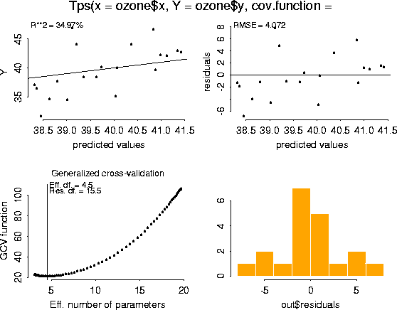
plot( ozone.tps)

Finally, here is the simplest example of using the predict function. The default is to predict at the observed data locations. ozone.tps.pred <- predict( ozone.tps)
ozone.tps.pred
 [1] 38.35702 38.62821 38.44499 39.01395 38.79481 39.72864 38.30791 39.35719
 [9] 39.19664 39.63307 40.98843 40.05890 41.11455 40.87318 41.42214 40.35936
[17] 40.03565 39.10773 41.34989 40.83722