A typical datafile

call it MinimalRadiosonde.txt

   Data Type:                     CLASS 10 SECOND DATA
   Launch Location (lon,lat,alt): 150 48.00'E, 02 35.00'S, 150.8, -2.58333, 3
   GMT Launch Time (y,m,d,h,m,s): 1993, 01, 17, 17:12:16
   Met Processor/Met Smoothing:   NCAR RS80 PROCESSOR, 10 SECONDS
   Winds Type/Processor/Smoothing:OMEGA, TRIMBLE MINI-OMEGA, 240 SECONDS
   Pre-launch Met Obs Source:     CAMPBELL SCIENTIFIC CR10
   /
   /
    Time  Press  Temp  Dewpt  RH   Uwind Vwind  Wspd  Dir     Lon     Lat
     sec    mb     C     C     %    m/s   m/s   m/s   deg     deg     deg
   ------ ------ ----- ----- ----- ----- ----- ----- ----- -------- -----
    -98.0 1004.9  24.2  23.7  97.0   0.0   0.0   0.0   3.8  150.800  -2.583
     10.0  999.8  26.0  24.7  92.4   0.0   -.1    .1  12.4  150.799  -2.586
    200.0  897.9  21.1  18.4  84.5   -.2   -.2    .3  50.6  150.799  -2.587
    710.0  699.1  10.9   5.9  71.1  -2.1  -1.3   2.4  58.6  150.796  -2.587
   1330.0  500.0  -5.0  -8.9  74.4  -1.0   2.4   2.6 157.8  150.792  -2.584
   1710.0  399.6 -13.6 -29.3  25.4  11.0    .7  11.0 266.2  150.799  -2.578
   2160.0  300.8 -28.9 -36.8  46.4   5.2  -3.0   6.0 300.2  150.829  -2.585
   2430.0  250.2 -39.5 -51.4  26.8   7.6   -.3   7.6 272.2  150.839  -2.590
   2730.0  200.9 -52.2 -61.1  33.4   9.1   2.7   9.5 253.3  150.860  -2.584
   3080.0  149.8 -67.3 -73.0  44.5   7.3   5.5   9.2 233.2  150.882  -2.573
   3510.0  100.2 -83.8 -88.7  43.0    .3   3.7   3.7 184.5  150.909  -2.557
   

Example

   filename <- "path/to/MinimalRadiosonde.txt"
   datakey  <- "------"
   varkey   <- " Time"
   unitkey  <- "  sec"
   sample.sonde <- getsonde(filename, datakey, varkey, unitkey)
   names(sample.sonde)
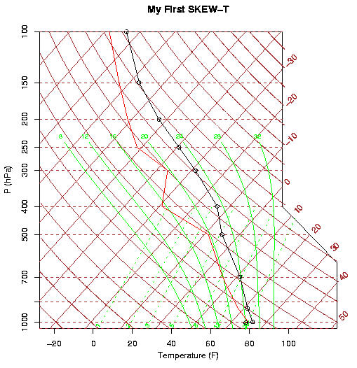
   plotsonde(sample.sonde,winds=F,title="My First SKEW-T")
   skewt.points(sample.sonde$temp,sample.sonde$press)
   attr(sample.sonde,"units")
   attr(sample.sonde,"metadata")
   

line-by-line explanation

1. filename... This line of the example simply builds a suitable filename.
   
   
2. datakey... This defines the character string that will be used to identify where the table of data starts in the radiosonde file. Rather than search for the first data entry, we search for the character string on the line BEFORE the data.IMPORTANT the string comparison will be conducted on only the initial characters on each line, therefore any initial whitespace is important! This is also true for varkey and unitkey
   
   
3. varkey... This defines the character string that will be used to extract the column names for the table in the radiosonde file.
   
   
4. unitkey... This defines the character string that will be used to extract the units of the observations or quantities. If there are no units, simply use unitkey = NULL
   
   
5. getsonde creates an R dataframe with named components that are the lower-case version of the values on the line started by varkey. If present, the header and units of the radisonde file are maintained as attributes of the dataframe.
   
   
6. names... This simply demonstrates how the component names of the dataframe are the lowercase version of the column headers in the original file. The result is

   [1] "time"  "press" "temp"  "dewpt" "rh"    "uwind" "vwind" "wspd"  "dir"  
   [10] "lon"   "lat"

7. plotsonde... This creates the standard SKEW-T, log P diagram used in the atmospheric science community.
   
   
8. skewt.points... Adds circles at the observation locations.
   
   
9. attr... simply echoes the "units" attribute. The result is

   [1] "sec" "mb"  "C"   "C"   "%"   "m/s" "m/s" "m/s" "deg" "deg" "deg"

10. attr... echoes the metadata; everything BEFORE the line containing the varkey.

The resulting SKEW-T, log p profile.

UCAR : NCAR : CISL : IMAGe : [  CMG   DAReS   GSP   RISC   TNT  ]
For problems with the page, contact Tim Hoar - thoar 'at' ucar 'dot' edu

© 2010, UCAR | Privacy Policy | Terms of Use | Contact UCAR | Visit UCAR | Sponsored by