|
|
|
| CISL | IMAGe | Statistics | Contact Us | Visit Us | People Search | |
|
Postdoctoral Opportunities in Statistics at the National Center for Atmospheric ResearchPostdoctoral appointments in statistics are a rather new phenomenon and the Geophysical Statistics Project (GSP) is unique among such programs. The quality of young statisticians in our project is extremely high. One strength of GSP is that it gives a new Ph D. the time to develop a solid research program of their own without the other pressures associated with the first few years as a faculty member. In addition, GSP provides a formative environment that encourages the post docs to branch out into new areas and develop applications in the geophysical and environmental sciences. The project is committed to maintaining NCAR connections with the statistics post docs after they leave. Thus, GSP post docs will retain their opportunities for collaboration with scientists here and also have the potential for funding outside the usual Probability and Statistics program at NSF.
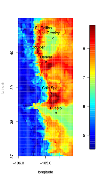
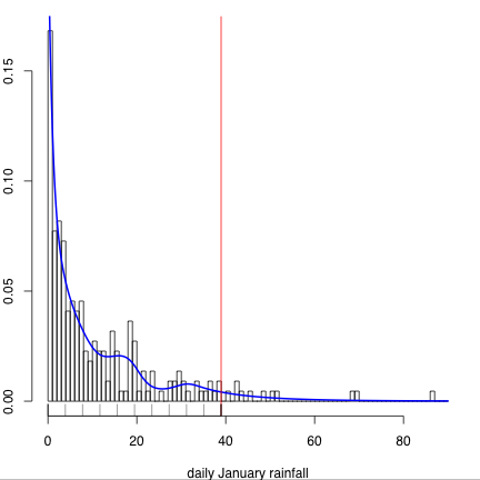
An Extreme Precipitation Return Levels Map for Colorado's Front RangeDan CooleyReturn levels maps are common tools used by flood planners to assess a location's potential for flooding by extreme precipitation events. The n-year return level is the (precipitation) amount which is exceeded on average once every n years. The maps supply information about potential extreme precipitation by providing return levels estimates for locations in the study region. Traditionally, these maps have not provided uncertainty estimates with the return levels. There is a current effort by the National Weather Service (NWS) to produce updated return levels maps. Using the Regional Frequency Analysis (RFA) methodology of Hosking and Wallis, the NWS has produced return levels maps and uncertainty estimates for two regions in the US. We have developed an alternative methodology to produce precipitation return levels maps along with uncertainty estimates. Our method differs from regional frequency analysis (RFA) in that it does not require predefined "homogeneous" regions in which to pool the data. Additionally, the parameters which describe the characteristics of the extreme precipitation are allowed to vary spatially via a geostatistical model. This suggests a natural way to interpolate from the station locations over study regions with very diverse precipation patterns. Using this methodology, we have produced a precipitation map for the Front Range region of Colorado, which consists of both mountains and plains. To construct the map, we have developed a three layer Bayesian hierarchical model which relies on the theory of extreme values. In the 'data layer', we model precipitation above a high threshold at 56 weather stations with the generalized Pareto distribution (GPD). The 'process layer' uses geostatistics methods to model the hidden process which drives extreme precipitation for the region. In this layer the GPD parameters are modeled as a Gaussian process. A 'prior layer' completes the model and priors are chosen to be relatively uninformative, which has the effect of not restricting the results to preconcieved solutions. An iterative algorithm (Markov Chain Monte Carlo) allows us to obtain successively more refined estimates of the precipitation returns levels. After many iterations (draws), the model parameter estimates stabilize and a collection of returns levels (the draws) is accumulated. These draws yield a natural method for obtaining uncertainty estimates for the precipitation return levels. The flexibility of the Bayesian hierarchical structure allows us to test different models which can be compared. Currently, we are working to extend the model to account for rainfall of different duration periods (e.g 6-hour and 12-hour rainfall amounts).
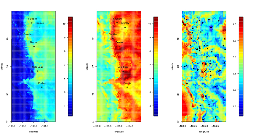
Caption for figure 2: Quantifying uncertainty. The left plot is the .025 quantile of the posterior distribution and could be used as a lower bound for the 25-year return level estimate. Similarly, the center plot is the .975 quantile and can be used as an upper bound. The right plot is the difference of the two, and thus shows the range of the 95% credible interval. The right panel also has black dots at the locations of the stations providing data for the analysis. The units are centimeters of precipitation per day (cm/day). This work is a collaboration with Doug Nychka, NCAR, and Philippe Naveau who has a joint appointment between Laboratoire des Sciences du Climat et de l'Environnement, IPSL-CNRS, Gif-sur-Yvette, France and Department of Applied Mathematics, CU Boulder Estimation of Climate Model ParametersDorin DrigneiA climate model is a mathematical model that describes the physical properties of climate variables such as temperature and precipitation over long time periods (e.g. decades or centuries). These mathematical models depend on parameters, some of which may be unknown or poorly known. The main theme of this research project is to estimate three such parameters: the climate sensitivity (S) defined as the change in global mean temperature due to doubling of atmospheric CO_2 concentrations, the global-mean vertical thermal diffusivity for the mixing of thermal anomalies into the deep ocean (K_v), and the net aerosol forcing (F_aer). By estimating appropriate values of these parameters, the climate model should more closely behave like the real climate system. The Massachusetts Institute of Technology (MIT) 2D climate model was run for many combinations of parameter values to generate a suite of results that will be used as a training set of parameter settings and the resulting climate quantities of interest. The statistical model being developed here is one that will recreate the climate quantities for the given parameter settings but will be sufficiently fast that a vast number of parameter combinations may be explored. This work is a novel implementation of new methodology called "Design and Analysis of Computer Experiments" (DACE). The fundamental tenet is that some computer experiments will always be too expensive to run, so one must be judicious in the experiments that are run. The novel aspect of this analysis is that the proposed statistical model takes into account the space-time correlations of the observational data and accounts for various sources of uncertainty, e.g., climate model internal variability, observational error, the difference in the behavior of the surrogate model and the original model, and so on. This results in much more accurate confidence intervals of the parameter of interest. The first two panels show the range and probablility for the climate sensitivity S and the thermal diffusivity K_v, while the third panel is the joint probability of S and K_v. The 95% confidence intervals for the first two panels are indicated by the diamonds. The 99% confidence interval is indicated by the squares. Compared to other methods (not shown), the confidence intervals appear to be shorter, indicating a more precise estimation method. More information is available at http://www.image.ucar.edu/~drignei. This is joint work with Doug Nychka of NCAR and Chris Forest of MIT. 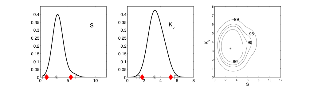
Figure 1. Left and middle panels: maximum likelihood estimates (star),
univariate kernel density estimates, 95% (diamond) and 99% (square)
confidence intervals for S and K_v;
Right panel: maximum likelihood estimates (star) and
bivariate kernel density estimates with contours representing
80, 90, 95 and 99% confidence regions for (S,K_v).
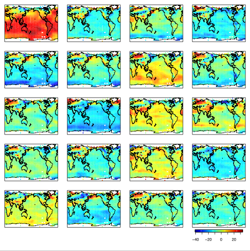
Large Statistical Models for the Biases of IPCC Climate ModelsMikyoung JunPotential global climate change due to human activities has been recognized as a serious problem and much effort has been devoted to detect the climate change signal. In 1988, the Intergovernmental Panel on Climate Change (IPCC) has been established to assess the risk and the impact of the human-induced climate change. There are numerous research groups over the world that run their own numerical climate models following IPCC standards. These numerical models are based on complex physics, chemistry and sciences and they should provide global climate "maps" not only for the current climate but also for past and future climates. Since these numerical models involve approximations, they may have biases, and the biases of each climate models are likely not the same. A common assumption in the study of climate models is that if we have enough climate models, their average should tend to the true climate and the biases of the climate models are independent of each other. If the biases are not independent from model to model, drawing inferences from the comparisons and determining the confidence bands of our predictions becomes much harder. Our interest is to build comprehensive statistical models that can jointly model all the climate model outputs and, through the statistical models, verify our conjecture that the above assumption of independent biases is not valid. Particularly, our statistical model should give correlations of the biases of climate models, so that we can classify the climate models into groups that share highly correlated biases. Our analysis is done on the surface temperature fields from 20 different IPCC climate models (figure 1 clearly illustrates the range of temperature fields from the different models). Our preliminary results identify subgroups of climate models that have highly correlated biases.
More details will be available at http://stat.tamu.edu/~mjun. This project is joint work with Reto Knutti and Doug Nychka of the National Center for Atmospheric Research. Ensemble Data AssimilationShree Prakash Khare
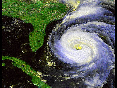
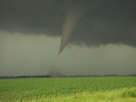
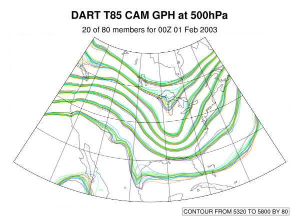
The earths atmosphere gives rise to a variety of phenomena like winter storms, hurricanes and tornadoes. The latter two phenomena are depicted in the above two figures. Making accurate forecasts of such phenomena is not only critical to the worldwide economy, but impacts peoples daily lives in a variety of ways. Physics, mathematics and computer science can be used to make predictions of weather phenomena. From classical laws of physics, accurate theories that describe the time evolution of the earths' atmosphere-ocean system can be derived. Mathematics and computers can be used to solve the equations derived from such physical theories. This mix of physics, mathematics and computer science results in a computer simulation model of weather phenomena. In order to make an accurate prediction of tomorrows weather, it is necessary to have a reasonably accurate idea of what todays weather looks like in order to 'initialize' the computer forecast model correctly. We can obtain information regarding todays weather by taking observations using a variety of weather stations placed on the earths surface and on satellites. Tiny changes in the initial conditions can cause the model to follow different paths and result in different estimates of the state of the atmosphere at some future time. In order to understand the effect of these unknowable uncertainties in the initial conditions, it is possible to run the models many times, starting from slightly different initial conditions and running up to the same forecast time. The end state of the model runs can be compared to get confidence limits that are useful for weather forecasters, for example, pinning down the most likely track of a hurricane. There are many applications for a group or ensemble of weather forecasts; not only is it is possible to give the most likely forecast, it is also possible to give the probability of the unlikely scenarios. There are many industries that are much more keenly interested in the occurrence of unusual weather events than the most likely weather events. For example, if half the models predict a moderate storm, but 25% of the models predict a particularly severe storm, it might be too risky for the fishing fleet to leave the harbor.
The procedure of combining observations and computer simulation models is known as data assimilation. The science of data assimilation tries to determine the 'optimal' way to combine prediction models and observations to address a number of questions of interest such as: Two days from now, what is the probability that the temperature in Boulder, Colorado will exceed 70F? The Geophysical Statists Project and the Data Assimilation Research Section of the National Center for Atmospheric Research have been working on data assimilation methods that provide highly accurate initial conditions that are consistent with the observations. Specific information and software is available at www.image.ucar.edu/DAReS. In the past year, we have shown a new approach, called 'Indistinguishable States', to be superior to a state-of-the-art 'Ensemble Kalman Filter' for solving the problem of data assimilation using probabilistic tests in a hierarchy of simple chaotic dynamical systems. As well, we have implemented and tested an 'Ensemble Smoother' tool that can be used retrospectively to obtain accurate estimates of the atmospheric state given all available observations in the past. The following website contains papers that address these topics, in addition to a variety of other ensemble data assimilation topics: www.image.ucar.edu/~khare. This is joint work with Jeff Anderson (DAReS), Doug Nychka (GSP), and Tim Hoar(GSP/DAReS).Space-Time Modeling of Atmospheric Carbon MonoxideAnders Malmberg, IMAGe, NCARwith Chris Wikle, Department of Statistics, University of Missouri, Doug Nychka, IMAGe, NCAR, and, David Edwards, ACD, NCARCarbon Monoxide (CO) is produced by incomplete combustion of carbon and carbon related materials, for example, in automobile engines and industrial processes. In concentrated amounts it is toxic and can cause death in a short time, and further, CO is a greenhouse gas that contributes to global warming. Therefore, CO indicates the air quality and it is an important gas for studying climate change. CO is also one of the few atmospheric species that can be remotely sensed from space. The Measurement of Pollution in the Troposphere (MOPITT) instrument, on the polar-orbiting Terra satellite, provides estimates of CO concentrations at seven different levels throughout the lowermost portion of the atmosphere. MOPITT collects data in swaths as it orbits the Earth, and over time covers nearly the entire globe. In any one day, however, there are gaps in the areas sampled by the satellite. This problem is ubiquitous for polar-orbiting sensors and is a major obstacle to researchers studying the time evolution of short-lived, rapidly-changing, or small-scale phenomena. 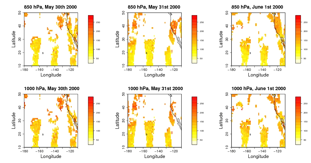
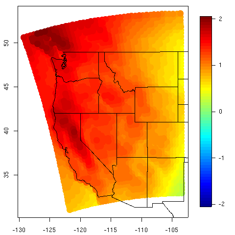
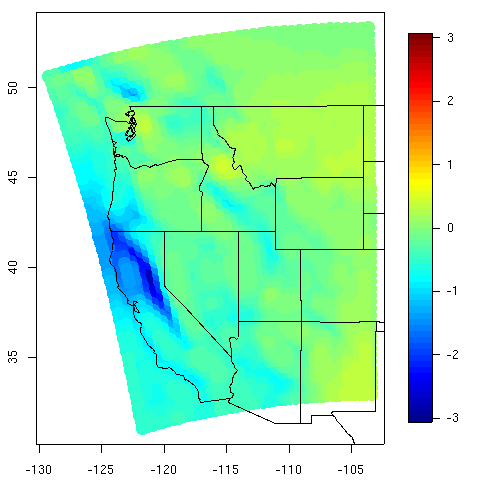
The figure shows the satellite-derived CO concentrations over a three day period for two vertical levels. The region depicted is the North Pacific Ocean from the West coast of the U.S. to the dateline. The bottom row of images is essentially at the surface of the earth (1000 hPa), the top row is a bit higher (850 hPa). The panels on the left are from a day before the panels in the middle, which are a day before the panels on the right. The bands of CO concentrations collected by MOPITT are clearly visible, while the gaps of no data are equally visible. Not only do the concentrations change from day-to-day, but the areas measured by MOPITT change daily. The concentrations are given in parts per billion. The goal of this study is to model the transport and chemical transformation of CO. However, to estimate a transport model and make air quality predictions, one has to consider that the data is sparse both in space and in time, and that there are additional sources of uncertainty in the data. The method is also expected to be broadly useful for many kinds of satellite observations, recognizing that the exact form of the model will need to be adapted for different phenomena. In this study we will break down the problem in stages, where the first stage is to model the data assuming that the true concentration is known; and then modeling the true concentration with some assumptions. The final stage is to make the assumptions sufficiently broad so as to encompass all likely possibilities. The assumptions are refined by running the model many times, where the ouput of the model from one run is used as the input to the model for the next run. This parameter estimation technique is called Markov Chain Monte Carlo (MCMC). Estimating the true CO mixing ratio and its dynamics will, in the end, allow us to make predictions of CO for the entire spatial domain for the entire timeframe of interest, as well as specifying the uncertainties of those predictions. Climate ChangeStephan Sain, Reinhard FurrerThe U.S. Climate Change Science Program Strategic Plan has recognized the need for regional climate modeling to assess climate impacts. This is the focus of the newly formed North American Regional Climate Change Assessment Program (NARCCAP) that seeks to study a number of regional climate models (RCMs). One goal of the statisticians in the program is to provide a general framework for synthesizing model output to obtain predictions of climate change and examine sources of variation in the different RCMs. At the heart of this framework is the development of multivariate spatial models. Recognizing the lattice structure present in climate model output, initial efforts have focused on the development of multivariate versions of Markov random field models, in particular Gaussian conditional autoregressive models. These models allow a very general and possibly asymmetric form of spatial dependence between the observed variables. To this end, new conditions on the parameters of such models have been established that ensure that the covariance structure of such models satisfy requirements to be bona fide covariance matrices. Incorporating this multivariate conditional autoregressive model in the specification of a spatial hierarchical model, we have begun to analyze output from a particular experiment involving the MM5 RCM driven by the NCAR/DOE Parallel Climate Model. The domain of the experiment was the western U.S. and the model used a 'business as usual' climate scenario (1% annual increase in greenhouse gasses). A four variable (winter and summer temperature and precipitation) version of the hierarchical model was fit using differences between 10-year averages (1995-2004 and 2040-2049). Bayesian computational methods (Markov chain Monte Carlo) were used to probe the posterior distributions of the parameters and the average climate change. Plots of the posterior mean climate change over winter months are shown.
Figure caption: Predictions of the average change in wintertime temperature (degrees Kelvin, left) and wintertime precipitation amount (inches of rain). Snow amounts are converted to equivalent rain amounts. This project involves a collaboration between Stephan Sain (University of Colorado at Denver), Reinhard Furrer (Colorado School of Mines), Noel Cressie (The Ohio State University), Doug Nychka (National Center for Atmospheric Research) and Linda Mearns (National Center for Atmospheric Research). Extreme Event Density EstimationStephan SainWeather generators that reproduce observed weather patterns can be useful tools for assessing, for example, the sources of variations affecting crop yields as well as the impacts of climate and climate change. At the heart of most weather generators is a probabilistic mechanism that can simulate temporal sequences of rainfall and temperature corresponding with seasonal patterns. However, it is often difficult to accurately reproduce extremes in temperature and weather, which are often the most influential factors for such things as crop failures, for example. Our goal is to develop a method for estimating the frequency(density) of observed weather quantities in a manner that retains important information about the extremes and that can be easily incorporated into current weather generators. Nonparametric density estimators are often plagued by difficulties in estimating the tails of distributions where data are scarce. This especially true of kernel methods. Logspline estimators are promising, but the knot selection strategies commonly employed move most of the knots to where there is more data (near modes) leaving the tail of the observed data to be modeled by what is effectively an exponential tail. We seek to improve on these approaches by creating a hybrid density estimator that uses a log-spline estimator near the modes with a parametric model based on the generalized Pareto density (GPD) for exceedances above a threshold for the tail. Constraints are incorporated to ensure that the resulting function is actually a valid density and that the density estimate is continuous and smooth (continuous first and second derivatives) at the breakpoint between the log-spline estimator and the GPD. We avoid knot the knot selection problem by using a moderate number of equally spaced knots and then using a type of penalized maximum likelihood. The penalty is based on enforcing smooth transitions between the coefficients of the logspline.
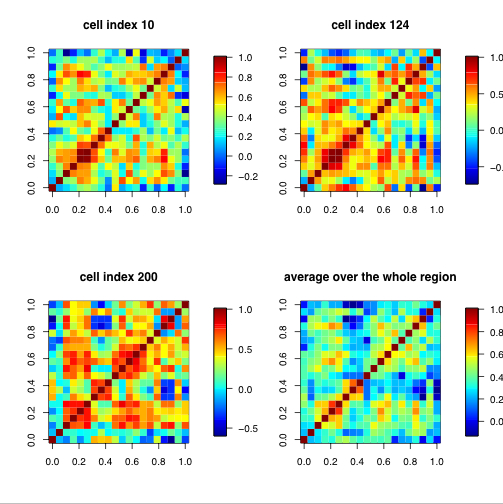
This project involves a collaboration between Stephan Sain (University of Colorado at Denver) and Doug Nychka (National Center for Atmospheric Research). Linda Mearns (National Center for Atmospheric Research) is also involved in the project. Nonstationary Covariance Modeling Using WaveletsTomoko MatsuoMonitoring air quality in the U.S. is accomplished through a network of local state and federal stations that are pooled to produce regional inferences on pollution. These stations are irregularly located and the coverage is sparse. Although the compliance of an urban area for air quality is primarily based on the station measurements, quantifying the exposure of a population to high ozone levels (for example) across a broader area requires a spatial analysis of the point monitoring data. If the ozone levels can be well predicted just by knowing the distance between two stations, statisticians would characterize ozone as having a stationary covariance. The covariance is needed to predict the ozone at unobserved locations and provide a measure of uncertainty of those predictions. However, daily surface ozone is well known to have nonstationary covariance over large regions and so standard geostatistics based on assumptions of stationarity are not appropriate. Techniques that require a complete gridded network of observation stations are similarly inappropriate. This work uses a mathematical construct called wavelets to create a model for the covariance that is a set of self-similar mathematical functions. Each wavelet only contains information for a limited area, so we use many of them. If there are N different wavelets, there are N*N combinations of wavelets needed to fully describe the covariance. Because of the limited region represented by a wavelet, some of the combinations are not needed. We have found that an excellent representation of the nonstationary covariance can be achieved using order N (not all N*N) combinations of wavelets. The appropriate wavelet combinations are chosen by determining the significant correlations among the wavelet coefficients. This can be justified from theory and has the practical benefit that the statistical computations can still be done efficiently. The figure displays the estimated covariance of surface ozone of the Eastern U.S. between the grid point indicated by the red dot and the rest of grid points for four sample locations. Figure(a) exhibits nonstationary spatial structure: an elongated correlation pattern along the urban coastal area. Figure(b) demonstrates a rather isotropic (i.e. radially symmetric) pattern in the midwest. There are two notable accomplishment of our work. The nonstationary covariance description is obtained with significant computational efficiency due to judicously retaining a small number of wavelet combinations and can be obtained from sparse and scattered observation locations. The illustration presented here had observations at only 364 of the 2304 total grid locations. In this case, our N is 2304, so N*N is more than five million. We only need about five thousand wavelet combinations to represent the nonstationary covariance. 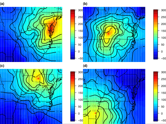
Figure caption: Non-stationary covariance for the Eastern U.S. obtained after the analysis of the daily maximum value of an 8-hour running mean ground-level ozone (184 days in May-Oct, 1997). [square of parts per billion (ppb^2)]
© 2010, UCAR |
Privacy Policy |
Terms of Use |
Contact UCAR | Visit UCAR |
Sponsored by
|