where f(X) is a d dimensional surface, and the object is to fit a thin plate spline surface to irregularly spaced data, e are random errors with zero mean, uncorrelated and with variances
 /W_i. A
mathematical summary of this type of spline is given in the last section of this
manual.
/W_i. A
mathematical summary of this type of spline is given in the last section of this
manual.
2.2 Cross-Validation
 , a parameter
controlling the amount of smoothing. For the case of one dimension and
m = 2, the estimate reduces to the usual cubic
spline.
, varies from zero
to infinity. When = 0 the spline estimate
interpolates the data and has a residual sums of squares of zero. At the other
extreme, of infinity results in an estimate that
is a polynomial of degree m - 1 with the
coefficients estimated by least squares. can be
chosen from the data by Generalized Cross-Validation (GCV). That is, the
estimate of the smoothing parameter can be found by minimizing the GCV function
) = N / D
, a parameter
controlling the amount of smoothing. For the case of one dimension and
m = 2, the estimate reduces to the usual cubic
spline.
, varies from zero
to infinity. When = 0 the spline estimate
interpolates the data and has a residual sums of squares of zero. At the other
extreme, of infinity results in an estimate that
is a polynomial of degree m - 1 with the
coefficients estimated by least squares. can be
chosen from the data by Generalized Cross-Validation (GCV). That is, the
estimate of the smoothing parameter can be found by minimizing the GCV function
) = N / D
where N = (1/n) * Y' (I - A(
))' W (I - A())Y and
D = (1 - trA()
/n)^2. Here, Y' denotes Y transposed, etc... It is also possible to include a
cost parameter that can give more (or less) weight to the effective number of
parameters beyond the base polynomial model.
, is found using the estimate for
by
= Y' (I - A())' W
(I - A())Y / (n -
tr(A())).
An alternate estimate is by maximum likelihood (see mathematical section).
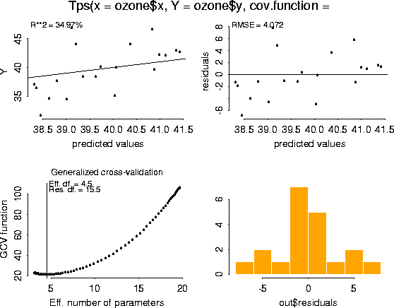
2.3 Tps Example: ozone
ozone.tps <- Tps( ozone$x, ozone$y)
summary( ozone.tps)


Call:

Tps(x = ozone$x, Y = ozone$y, cov.function =
 "Thin plate spline radial basis functions (rad.cov) ")
1. Number of Observations: 2. Number of unique points: 3. Degree of polynomial null space ( base model): 4. Number of parameters in the null space 5. Effective degrees of freedom: 6. Residual degrees of freedom: 7. MLE sigma 8. GCV est. sigma 9. MLE rho 10. Scale used for covariance (rho) 11. Scale used for nugget (sigma^2) 12. lambda (sigma2/rho) 13. Cost in GCV 14. GCV Minimum |
20 20 1 3 4.5 15.5 4.098 4.072 205.8 205.8 16.79 0.0816 1 21.41 |
 Residuals:
    min  1st Q  median 3rd Q   max
 -6.801 -1.434 -0.5055 1.439 7.791
 REMARKS
Covariance function: rad.cov
-
1. the total number of
observations including replicates.
2. the total number of unique points.
3. the maximum degree of polynomial (m - 1) included in the spline model.
4. total number of polynomial terms up to the maximum degree. This is the total number of conventional parameters for the spline.
5. total number of effective parameters associated with the spline curve including those of the polynomial. This number is controlled by the parameter
and is the trace
of the smoothing matrix, A(). 6. spline degrees of freedom subtracted from the total number of observations.
7. estimate of
by maximum likelihood. 8. estimate of
by using residual sum of squares and effective
d.f. 9. - 11. these are explained in the discussion of the Krig function and the spatial model.
12. value of smoothing parameter used to find spline estimate. If no value has been specified, the smoothing parameter estimated by GCV is reported.
13. value of cost parameter.
14. value of GCV function at
. This is an estimate of the average squared
prediction error for a given value of . If
has been estimated, then the minimum value of the
GCV function is reported.
plot( ozone.tps)
Finally, here is the simplest example of using the predict function. The default is to predict at the observed data locations. ozone.tps.pred <- predict( ozone.tps)
ozone.tps.pred
 [1] 38.35702 38.62821 38.44499 39.01395 38.79481 39.72864 38.30791 39.35719
 [9] 39.19664 39.63307 40.98843 40.05890 41.11455 40.87318 41.42214 40.35936
[17] 40.03565 39.10773 41.34989 40.83722
Back to top
3. Spatial Process Models: Krig
where P is a low order polynomial (default polynomial used by Krig is a linear function (m=2)). Z is a mean zero, Gaussian stochastic process with a covariance that is known up to a scale constant,
 k(x, x') and denote the variance
of e_i by /W_i. Consistent with the spline estimate, we take
= /
. The covariance function, k, may also depend
on other parameters that we explain how to specify below but these are not estimated directly by the Krig function.
k(x, x') and denote the variance
of e_i by /W_i. Consistent with the spline estimate, we take
= /
. The covariance function, k, may also depend
on other parameters that we explain how to specify below but these are not estimated directly by the Krig function.
3.1 Using Krig
, is found by GCV. If one assumes a Gaussian
process and Gaussian errors, then this estimate is also related to the
conditional expectation of f(x) given the observed data. Of equal value are
estimates of the standard errors of prediction and more will be said about these
below. where rdist( x, x') is the Euclidean distance function and the default for theta is 1. To set parameters of the covariance function to values other than their defaults, simply include them in the calling list to Krig. The example below indicates how this is done.
fit <- Krig( ozone$x, ozone$y, theta=100)
3.2 Examples
The following examples illustrate the use of Krig and supporting functions.
-
Ozone data example.
Ozone Concentrations in Chicago
- Overall Plots of the Data (and how to create them)
- Krig fit with exponential covariance function
- Summary of above fit
- Diagnostic plots of the Krig fit
- Prediction Standard Errors
- Predicting (on and off the data)
-
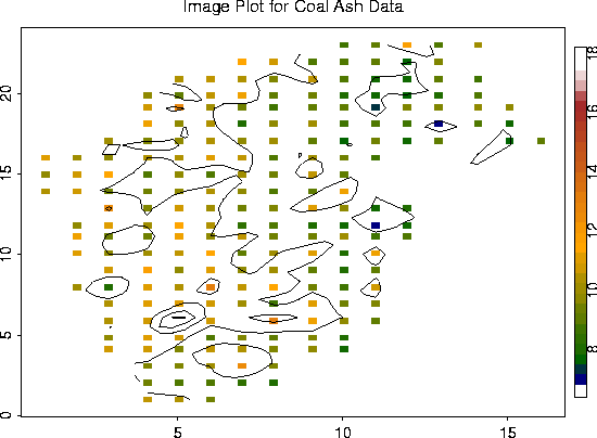
Coal-ash data example.
(Data obtained from Gomez and Hazen (1970, Tables 19 and 20) on coal ash for the Robena Mine Property in Greene County Pennsylvania.)
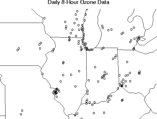
- Daily 8-hour Ozone data
Daily 8-hour surface ozone measurements during the summer of 1987 for approximately 150 locations in the Midwest.
Back to top
Ozone Concentrations in Chicago
Although not a very interesting data set, it is useful for demonstrating the Krig package.
Overall plots of the data:
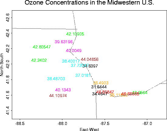 Close-up |
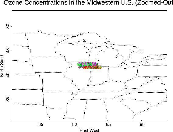 Zoomed-out (to see location better) |
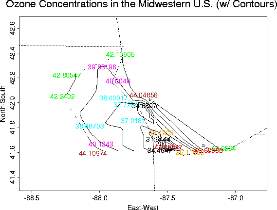 Contour Plot |
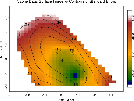
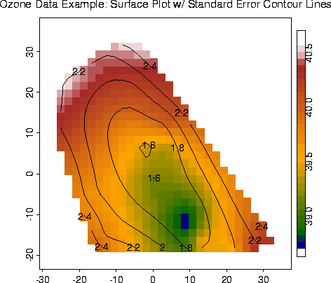 Surface Plot w/ Standard Errors from Krig fit |
# -- Find the Krig fit to the ozone data using
# -- Exponential covariance function. Choice of range parameter, theta, is
# -- arbitrarily chosen here to be 10 miles.
fit <- Krig(ozone$x, ozone$y, exp.cov, theta=10)
# -- Print summary of the Krig fit.
# -- The summary function is a generic S-Plus function that is used to provide
# -- summary information about a regression object. For example, from the
# -- output of the summary below, we can discern that 4 or 5 parameters
# -- (Effective df=4.5) are needed to fit the model. Also, the estimate for
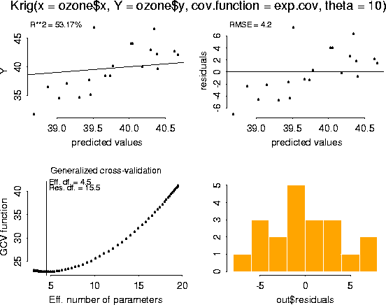
# -- sigma is about 4.2 (both MLE and GCV give this), and for rho is 2.374.
summary( fit)
Call:
Krig(x = ozone$x, Y = ozone$y, cov.function = exp.cov, theta = 10)


Number of Observations:				20
Number of unique points:			20
Degree of polynomial null space ( base model):  1
Number of parameters in the null space		3
Effective degrees of freedom:			4.5
Residual degrees of freedom:			15.5
MLE sigma					4.206
GCV est. sigma					4.2
MLE rho						2.374
Scale used for covariance (rho)			2.374
Scale used for nugget (sigma^2)			17.69
lambda (sigma2/rho)				7.453
Cost in GCV					1
GCV Minimum					22.8

 Residuals:
    min  1st Q  median 3rd Q   max
 -7.037 -2.189 -0.4681 2.299 7.382
 REMARKS
Covariance function: exp.cov
# -- Obtain diagnostic plots of the fit using the generic function, plot.
# -- This is the same function used for other standard S-Plus regression
# -- objects. Note that the plots of the residuals suggest that the model is
# -- overfitting ozone at lower values.
plot( fit)
# -- Calculate the standard errors of the Krig fit using the Fields function
# -- predict.se.Krig, which finds the standard errors of prediction based on a linear
# -- combination of the observed data--generally the BLUE. The only required
# -- argument is the Krig object itself. Optional arguments include alternate
# -- points to compute the standard error on, viz. x, a covariance function, rho, sigma2
# -- (default is to use the values passed into Krig originally),
# -- and some other logical parameters that can be found in the help file.
ozone.fit.se <- predict.se( fit)
out.p <- predict.surface( fit)
image.plot( out.p, xlab="East-West", ylab="North-South")
out2.p <- predict.surface.se( fit)
contour( out2.p, add=T)
# -- It is also possible to obtain krig predictions at other locations besides
# -- those given with the data. For example,
# -- Here, I choose a random set of points to predict at. I did this to
# -- emphasize that you can choose any grid points that you want
# -- to study.
loc.knot <- cbind (runif( 20, min=-30, max=35), runif( 20, min=21, max=36))
# -- Now predict with these points.
ozone.pred2 <- predict( fit, loc.knots)
# -- We can also use predict to obtain predictions for the ozone fit using a
# -- different value for lambda, or df--and, indeed, different data.
# -- For example,
ozone.pred3 <- predict( fit, lambda=5)
Back to top
Data obtained from Gomez and Hazen (1970, Tables 19 and 20) on coal ash for the Robena Mine Property in Greene County Pennsylvania.
Overall plot of the data.
# -- Create an image plot of the data. For fun, add the contour lines.
look <- as.image( coalash$y, x=coalash$x)
image.plot( look)
contour( look, add=T, labex=0)
# -- Perform a Krig fit using exponential covariance function with range
# -- paramter, theta=2.5 (choice of theta will be explained below).
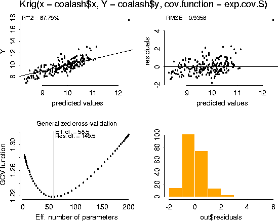
fit <- Krig( coalash$x, coalash$y, cov.function = exp.cov.S, theta=2.5)
summary( fit)
Call:

Krig(x = coalash$x, Y = coalash$y, cov.function = exp.cov.S)


Number of Observations:                        208
Number of unique points:                       208
Degree of polynomial null space ( base model): 1
Number of parameters in the null space         3
Effective degrees of freedom:                  29.7
Residual degrees of freedom:                   178.3
MLE sigma                                      1.02
GCV est. sigma                                 1.018
MLE rho                                        0.2829
Scale used for covariance (rho)                0.2829
Scale used for nugget (sigma^2)                1.04
lambda (sigma2/rho)                            3.675

RESIDUAL SUMMARY:
    min   1st Q   median  3rd Q   max
 -2.169 -0.6578 -0.09917 0.4115 6.169

COVARIANCE MODEL: exp.cov.S

DETAILS ON SMOOTHING PARAMETER:
 Method used:   GCV    Cost:  1
 lambda   trA   GCV GCV.one GCV.model  shat
  3.675 29.69 1.209   1.209        NA 1.018

 Summary of estimates for lambda
        lambda   trA   GCV  shat
    GCV  3.675 29.69 1.209 1.018
GCV.one  3.675 29.69 1.209 1.018
plot( fit)
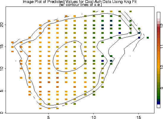
# -- We will use the S-Plus generic function, predict, to make predictions,
# -- using the Krig object fit.
# -- We also added the contours of the standard errors of the estimates.
fit.pred <- predict( fit)
look <- as.image( fit.pred, x=coalash$x)
image.plot( look)
fit.se <- predict.se( fit)
look2 <- as.image (fit.se, x=coalash$x)
contour( look2, add=T, labex=0)
| theta | GCV Minimum |
0.5 0.75 1.0 1.25 1.5 1.75 2.0 2.25 2.5 2.75 3.0 3.25 3.5 3.75 4.0 4.25 5.0 10.0 100.0 |
1.225 1.221 1.218 1.216 1.214 1.212 1.211 1.21 1.209 1.209 1.208 1.208 1.207 1.207 1.207 1.207 1.206 1.205 1.205 |
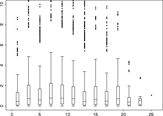
coalash.vgram <- vgram( coalash$x, coalash$y)
# -- coalash.vgram is a list object. Where "d" are the distances,
# -- coalash.vgram$vgram is the variogram, and call tells how the vgram function was called.
names( coalash.vgram)
[1] "d" "vgram" "call"
bplot.xy( coalash.vgram$d, coalash.vgram$vgram)
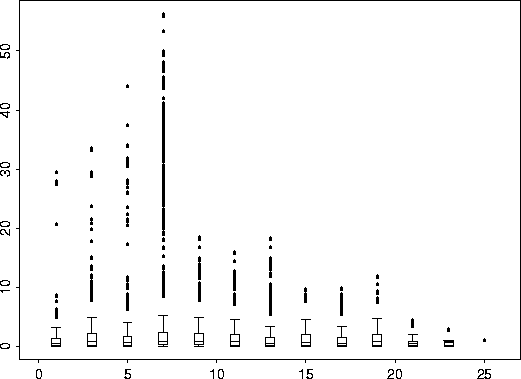 |
 |
Now we use the S-Plus function, nls (Non Linear Least Squares Regression) to search for a suitable range parameter. Simultaneously, we search for possible values for sigma2 and rho which we can subsequently fix, if desired, for the Krig fit. vgram.fit <- nls( vgram ~ sigma2*(1-rho*exp(-d/theta)), coalash.vgram, start=list( sigma2= 9, rho=0.95, theta=1)) summary( vgram.fit)
Formula: vgram ~ sigma2 * (1 - rho * exp( - d/theta))

Parameters:
          Value Std. Error  t value
sigma2 1.696190  0.0334569 50.69770
   rho 0.750553  0.2807990  2.67292
 theta 1.635050  0.5580010  2.93019

Residual standard error: 3.60828 on 21523 degrees of freedom

Correlation of Parameter Estimates:
      sigma2    rho
  rho -0.346
theta  0.566 -0.877
fit <- Krig( coalash$x, coalash$y, theta=1.635050, sigma2=1.696190, rho=0.750553)
summary( fit)
CALL:
Krig(x = coalash$x, Y = coalash$y, rho = 0.750553, sigma2 = 1.69619, theta =
        1.63505)

 Number of Observations:                        208
 Number of unique points:                       208
 Degree of polynomial null space ( base model): 1
 Number of parameters in the null space         3
 Effective degrees of freedom:                  48.8
 Residual degrees of freedom:                   159.2
 MLE sigma                                      0.9604
 GCV est. sigma                                 0.9647
 MLE rho                                        0.4082
 Scale used for covariance (rho)                0.7506
 Scale used for nugget (sigma^2)                1.696
 lambda (sigma2/rho)                            2.26

RESIDUAL SUMMARY:
    min   1st Q  median  3rd Q   max
 -1.899 -0.5541 -0.1009 0.3808 5.486

COVARIANCE MODEL: exp.cov

DETAILS ON SMOOTHING PARAMETER:
 Method used:   user    Cost:  1
 lambda  trA   GCV GCV.one GCV.model   shat
   2.26 48.8 1.216   1.216        NA 0.9647

 Summary of estimates for lambda
        lambda   trA   GCV   shat
    GCV  3.422 37.27 1.213 0.9979
GCV.one  3.422 37.27 1.213 0.9979
Back to top
The Fields dataset ozone2 consists of daily 8-hour surface ozone measurements during the summer of 1987 for approx. 150 locations in the Midwest.
# Plot the data with a map of the area.
usa( xlim= range( ozone2$lon.lat[,1]), ylim= range( ozone2$lon.lat[,2]))
points( ozone2$lon.lat, pch="o")
title("Daily 8-Hour Ozone Data", cex=0.85)
It will be handy to create a correlogram before we continue.
ozone.cor <- COR( ozone2$y)
mean.tps <- Tps( ozone2$lon.lat, ozone.cor$mean, return.matrices = F)
sd.tps <- Tps( ozone2$lon.lat, ozone.cor$sd, return.matrices = F)
day16 <- c( ozone2$y[16,])
# -- Logical vector to remove missing values from day16.
idn <- !is.na( day16)
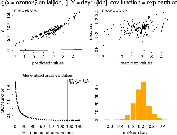
fit <- Krig( ozone2$lon.lat[idn, ], day16[idn], cov.function=exp.earth.cov, theta = 343, sd.obj=sd.tps, mean.obj=mean.tps, m=1) summary( fit)
Krig(x = ozone2$lon.lat[idn,  ], Y = day16[idn], cov.function = exp.earth.cov,
        m = 1, mean.obj = mean.tps, sd.obj = sd.tps, theta = 343)

 Number of Observations:                        147
 Number of unique points:                       147
 Degree of polynomial null space ( base model): 0
 Number of parameters in the null space         1
 Effective degrees of freedom:                  114.7
 Residual degrees of freedom:                   32.3
 MLE sigma                                      0.289
 GCV est. sigma                                 0.3172
 MLE rho                                        7.538
 Scale used for covariance (rho)                7.538
 Scale used for nugget (sigma^2)                0.0835
 lambda (sigma2/rho)                            0.01108
 Cost in GCV                                    1
 GCV Minimum                                    0.4585

Y is standardized before spatial estimate is found
 Residuals:
     min    1st Q   median   3rd Q   max
 -0.6091 -0.07774 0.003612 0.08233 0.433
 REMARKS
Covariance function: exp.earth.cov
Back to top
3.3 Covariance Functions
 my.cov <- function( x1, x2, p = 1, range=1) {
        cov <- exp( - (rdist(x1, x2)/range)^p)
        return( cov)
        }
Then, to use this function with Krig, simply include its name along with any parameters to be passed in. That is,
fit <- Krig( data$x, data$y, my.cov, range=12, p=1.5)
Back to top
| Table - Covariance functions in Fields | ||||
|---|---|---|---|---|
| Name/ description | S-Function | optional arguments with defaults | Fortran/S version | C argument |
| Exponential/ Gaussian | exp.cov | theta = 1, p = 1 | both | yes |
| Exponential for sphere | exp.earth.cov | theta = 1 | S | no |
| Matern | matern.cov | smoothness = 0.5 range = ?? | FORTRAN | no |
| Periodic 1-d | periodic.cov.ld | a = 0, b = 1 | both | no |
| Cylindrical | periodic.cov.cyl | a = 0, b = 365 theta = 1 | S | no |
| Poisson covariance for the sphere | poisson.cov | eta = 0.2 | S | no |
| Sample covariance | test.cov | theta = 1 | S | no |
| Generalized spline covariance | rad.cov | p | both | yes |
Back to top
3.4.2 Defining New Covariance Functions
foo.cov.S <- function( x1, x2, range) {

	exp( -(rdist(x1, x2)/range)**2)

} # end of foo.cov fcn (Note that foo.cov.S is the Gaussian covariance fcn.)
foo.fit <- Krig( ozone$x, ozone$y, cov.function=foo.cov.S, range=10)
summary( foo.fit)
Call:

Krig(x = ozone$x, Y = ozone$y, cov.function = foo.cov.S, range = 10)


Number of Observations:                        20
Number of unique points:		       20
Degree of polynomial null space ( base model): 1
Number of parameters in the null space         3
Effective degrees of freedom:                  3.2
Residual degrees of freedom:                   16.8
MLE sigma                                      4.402
GCV est. sigma                                 4.402
MLE rho                                        0.2765
Scale used for covariance (rho)                0.2765
Scale used for nugget (sigma^2)                19.38
lambda (sigma2/rho)                            70.08
Cost in GCV                                    1
GCV Minimum                                    23.06


Residuals:
    min  1st Q  median 3rd Q   max
 -7.802 -2.736 -0.3941 2.757 7.472
 REMARKS
Covariance function: foo.cov.S
Utilizing the C argument
This particular computation can be invoked using the C argument. That is,
The advantage is that Krig will not create the covariance matrix, Sigma. Instead, it will perform the calculations of Sigma %*% C using, in most cases (true for all Fields provided covariance functions), a Fortran subroutine and save only the result of the multiplication.
Back to top
3.4.3 Calling the Covariance Function by Name or by Function
(cov.by.name logical parameter)
What in the world does this parameter do?
do.call( out$call.name, c( out$args, list( x1, x2)))
may appear to be more complicated, but more compatible with the implementation of the S language in the R statistical package. Note that out$call.name is a character value that simply stores the name of the covariance function to be called. For example, if the default exp.cov is used, then out$call.name is "exp.cov".
Back to top
Some Details on Tps and Krig
Tps and Krig:
The Tps estimate can be thought of as a special case of a spatial process estimate using a particular generalized covariance function. Because of this correspondence the actual Tps function is a short wrapper that determines the polynomial order for the null space and then calls Krig with the radial basis generalized covariance (rad.cov). In this way Tps requires little extra coding beyond the Krig function itself and in fact the returned list from Tps is a Krig object and so it is adapted to all the special functions developed for this object format. One down side is some confusion in the summary of the thin plate spline as a spatial process type estimator. For example, the summary refers to a covariance model and maximum likelihood estimates. This is not something usually reported with a spline fit!
Replications
By a replicate point we mean more than one observation made at the same location. The Fields BD dataset is an example. The Tps and Krig functions will handle replicate points automatically, identifying replicated values and calculating the estimate of sigma based on a pure error sums of squares. The actual computation of the estimator is based on collapsing the data into a set of unique locations and the dependent vector y is collapsed into a smaller vector of weighted means. The Fields functions cat.matrix and fast.1way are used to efficiently identify the unique locations and produce the replicate group means and pooled weights. Replicate points posed several ways of performing cross-validation and this issue is discussed below.
Matrix decompositions
In writing Krig a decision was made that the Krig object can be used to find estimators for many different values of lambda (the ratio of sigma squared to rho). The computations to evaluate the estimator for many values of lambda are more extensive than for just one value. In this general case, the matrix computations are dominated the cube of the number of unique locations, np. The Wahba-Bates-Wendelberger algorithm (WBW) requires an eigenvector/eigenvalue of a matrix on the order np x np and the Demmler Reinsch algorithm (DR) requires the inverse square root and eigenvector/eigenvalue decompositions of np size matrices. Unlike WBW the DR is more amenable to using a reduced set of basis functions and so it is the default for Krig. However, for consistency with other spline implementations (e.g. GCVPACK) WBW is the default method for Tps. The user can control which is used by the decomp argument in the call.
Reducing the number of basis functions
The Krig estimate is a function that is a linear combination of basis functions derived from the covariance kernel. By default the standard Kriging estimator uses as many basis functions as unique locations. For large problems and noisy data this may be excessive. For example with 1000 locations one may feel that the true surface can be adequately approximated with far fewer degrees of freedom than that afforded by the full set of 1000 basis functions. To support this approximation, Krig and Tps have the option of taking a set of knot locations that define a basis independently of the data. The basis functions are bump shaped functions defined by the covariance and with the peak centered at the knot location. Thus evenly distributing the knot locations throughout the data region may be reasonable. One might also construct knot locations from a regular grid or use the cover.design function to find an irregular set of space filling points or just randomly sample (without replcement!) the observed data locations.
Here is an example for the Midwest ozone data.
#50 points selected from the locations that purposefully spread out.
knots <- cover.design( ozone2$lon.lat, 50)$design
good<- !is.na( ozone2$y[12,])
x<- ozone2$lon.lat[good,]
y<- c( ozone2$y[12,good])
Tps( x, y, knots=knots)-> out
[1] "Maximum likelihood estimates not found with knots \n \n "
The warning from this fit is expected because some estimates related to the covariance are not well defined for a reduced basis set.
Generalized cross-validation and choosing the smoothing parameter
The smoothing parameter, lambda is estimated by default by minimizing the generalized cross validation function. When there are no replicate points and full basis is used there is no ambiguity about the form for GCV. The basic CV strategy is to omit a part of the data and use the model fit on the remaining data to predict the left out observations. This basic form is the GCV.one criterion calculated in gcv.Krig. However, the GCV criterion is a ratio with the numerator being a mean residual sum of squares and the denominator being the squared fraction of degrees of freedom associated with the residuals. Variations on GCV used in Krig are based on modifying the mean square of the numerator and the number of observations entering the denominator.
For replicate points or a reduced set of basis functions the residual sums of squares can be broken into a pure error piece and one that is is changed by the smoothing parameter. For replicates this is the pure error sums of squares of the observations about their group means and for a reduced basis it is the residual sums of squares from regressing the full basis on the data. The default GCV criterion weights these pieces separately in an attempt to make the numerator more interpretable as an estimate of mean squared error.
With replicate points an alternative to omitting individual observations is to omit the entire replicate group. Technically this is accomplished by omitting the pure error sums of squares from the denominator of the GCV criterion. We refer to this result as GCV.model and is less likely to over fit the data than the other criterion.
The BD dataset in Fields contains replicated points. As an example, here are the results of different criterion applied to this data set.
fit <- Tps(BD[,1:4], BD$lnya, scale.type="range")
fit$lambda.est
Besides these three versions of the GCV criterion another point of flexibility is the cost parameter used in the denominator. The default is cost=1 although specifying larger costs will force the criterion to favor models with fewer model degrees of freedom. For the BD example we see:
gcv.Krig( fit, cost=2)$lambda.est
In the discussion given above it has been assumed that once a GCV criterion is adopted one seeks to find the lambda value that minimizes the criterion. We have two qualifications of this basic approach. First in any minimization it is a good idea to examine the criterion for multiple local minima and other strange behavior. The plot function applied to the Krig or Tps object will plot the GCV measures as a function of the smoothing parameter ( Usually the lower left plot in the panel of 4). It is a good idea to examine this graph. Secondly, with replicate points, one may want the estimate of sigma^2 implied by the curve or surface fit to agree with that obtained from the pure error estimate. So rather than minimize a GCV criterion one would find the value of lambda so that the two estimates of sigma^2 are equal. In terms of the Krig object this would find lambda so that shat.GCV and shat.pure.error are equal. The only hazard of this estimate is when the replicates give an artificially low representation of the error variance. One should also note that this equality is not always possible because the pure error estimate may be outside the range possible from the spline based estimate.
Reusing objects:
The overall strategy for the Krig and Tps function is to do some extensive matrix decomposition once and then exploit their use in finding the estimate at many different values of lambda or even different sets of observations. In particular the predict and gcv.Krig functions are not limited to just the estimated values of lambda and the data vector y used to create the Krig object. The only constraint is that if the locations of the observations or the weighting matrix for the error variance are changed, then decompositions must be redone. Besides being efficient for looking at different values of the smoothing parameter this setup also facilitates bootstrapping and simulation.
Here are some short examples to show how this works.
Tps(ozone$x, ozone$y)-> fit
the GCV estimate gives an effective degrees of freedom of around 4.5.
predict(fit)
evaluates the spline at this level of smoothing
predict( fit, df=8)
evaluates the spline using a model with the effective degrees of freedom is equal to 8. This last result is equivalent to
Tps(ozone$x, ozone$y, df=8)-> fit2
predict( fit2)
but is more efficient because the decompositions are not recreated. Instead they are reused from the fit object.
To redo the GCV search with new data one can just call gcv.Krig with the Krig object and another y,
gcv.Krig( fit, y=ozone$y)-> gcv.out
Here is an example of a bootstrap to see the sampling variability for GCV. Assume that the "true" function is the spline estimate from the data. We will reuse the Krig object to get efficient estimates when just the y's are changed.
true<- fit$fitted.values
sigma<- fit$shat.GCV
out<- matrix(NA, nrow=50, ncol=4)
set.seed(123)
for( k in 1:50){
y<- true + rnorm(20)*sigma
gcv.Krig( fit, y=y)-> temp
out[k,] <- temp$lambda.est[1,]
}
Within this loop we have just saved the estimated smoothing parameter. However, an additional line calling predict with the old object but the simulated data and new value of lambda would give an efficient evaluation of the estimated spline.
Finally a scatterplot of the results
plot( out[,2], out[,4], xlab="eff df", ylab="shat.GCV")
One moral from these results is to try different values of the smoothing parameter -- although GCV usually gives unbiased estimates, it is also highly variable.
Back to top
5.1 Space-Filling Designs
At this point an analogy may be helpful to explain the coverage criterion. Suppose that you are charged with locating a fixed number of convenience stores in a city. Given a particular set of store locations each resident will have a store that is closest to their home. Out of all the residents, find the one who is the farthest to their nearest store. This is the maximum over the nearest neighbor distances and a good design for the stores makes this criterion as small as possible. In words, one seeks to minimize the distance the residents must travel to their closest convenience store. The result is referred to as the minimax design.
The cover.design function has two approximations. The minimax criterion is approximated by a smoother criterion based on L_p norms. These are the P and Q arguments in the call. The defaults P=Q=32 appear to yield a good approximation to the minimax designs. The other approximation is that the coverage criterion is minimized by updating one design point at a time. For each design point one checks whether a swap with a candidate point will yield a smaller coverage criterion. If such a swap is found the swap is made: the new point is adopted as part of the design and the old design point is moved into the candidate set. This process continues until no more productive swaps can be made or the number of iterations is exceeded. This algorithm is not guaranteed to give a global minimum and so one may not obtain the optimal design solution. However, we have found this algorithm to give useful designs even if they are not the global minimizer. In general, the global minimum is difficult to find and has questionable added value over good approximate solutions.
There are several important features of the cover.design function related to the algorithm for finding the design. One can fix some points in the design. These are simply points that are not allowed to be swapped out. This is useful if one wants to build up a sequence of designs of increasing size with the smaller designs being subsets of the larger ones. The default is to use Euclidean metric to measure distance between points. Any S function that is a metric can be substituted for this choice. See the help file for an example. Finally the swapping algorithm may only consider swapping candidate points that are near neighbors of the design point. This is helpful when the candidate set is large.
Here is a simple example to thin out a random set of 2-d locations and shows how the fixed point option works.
Create 200 locations uniformly distributed in the unit square.
set.seed( 123)
cand <- matrix( runif( 200*2), ncol=2)
Now find a coverage design of 10 points
cover.design(cand, 10)-> design10
The component design10$design is the best design and design10$best.id gives the row numbers of the candidate set matrix that comprise the best design.
Check it out
plot( design10)
summary( design10)
Now add 20 more points for a total of 30
cover.design( cand, 30, fixed=design$best.id)
Here is what happened:
plot( cand, pch=".")
points( design10$design, pch="x", col=2)
points( design30$design, pch="o", col=3)
Back to top
By a surface or image object we mean a list with components x, y and z Where x and y are equally spaced grids and z is a matrix of values. This is the same format as used by the S functions contour, image, and persp
as.image creates an image object from irregular x,y,z by discretizing the 2-d locations to a grid and then producing an image object with the z values in the right cells. The arguments necessary for as.image to work are:
Z: Values of image.
The rest of the arguments are optional. They are:
- ind = NULL, A matrix giving the row and column subscripts for
each image value in Z. (Not needed if x is specified)
- grid = NULL, A list with components x and y of equally spaced
values describing the centers of the grid points. The default is to use
nrow and ncol and the ranges of the data locations (x) to construct a
grid.
- x = NULL, Locations of image values. Not needed if ind is
specified.
- nrow = 64, Number of rows in image matrix (x-axis direction).
- ncol = 64, Number of columns in image matrix
(y-axis direction)
- weights = rep( 1, length(Z))
look <- as.image( coalash$y, x = coalash$x)
image.plot (look)
In this conversion grid boxes without Z value are coded as NA and so appear as the background color in an image plot. The function image.plot has the same functionality as image but adds a legend strip. It can be used to add a legend strip to an existing plot or create a new image and legend. Its chief benefit is that this function resides the plot region automatically to make room for the legend strip. We have found a function with reasonable defaults has been quite useful.
Back to top
- Cressie, Noel A.C. (1993). Statistics for Spatial Data Wiley, USA.
- Gomez, M. and Hazen, K. (1970). Evaluating sulfur and ash
distribution in coal seems by statistical response surface regression
analysis. U.S. Bureau of Mines Report RI 7377.
- Isaacs, Edward H. and Srivastava, R. Mohan (1989). An
Introduction to Applied Geostatistics. Oxford University Press, NY.
- Journel, A.G. and Huijbregts, C.J. (1978). Mining Geostatistics
. Academic Press, London.
- Nychka, D. (1998). Spatial Process Estimates as Smoothers.
Smoothing and Regression. Approaches, Computation and Application
ed. M. G. Schimek, Wiley, New York.
- Nychka, D., Piegorsch, Walter W., and Cox, Lawrence H. (Editors)
Case Studies in Environmental Statistics (1998) Springer, NY.
- Ripley, Brian D. (1981). Spatial Statistics Wiley, NY.
- Venables, W.N. and Ripley, B.D. (1994). Modern Applied Statistics with S-Plus Springer-Verlag, NY.
Back to top