Fields: On-Line Manual

[an error occurred while processing this directive]

Fields: Web Manual
Table of Contents

1. Introduction

2. Thin Plate Splines: Tps

3. Spatial Process Models: Krig

4. Simulating Random Fields (sim.rf)

5. Spatial Predictions for Large Data Sets

6. Other Fields Functions

Space-Filling Designs
Working With Images
- Gridding Irregular Spaced Observations
- Smoothing Images
- Plotting

References

Printable version of Fields Manual

Back to Fields Home Page

Coal Ash Data Example
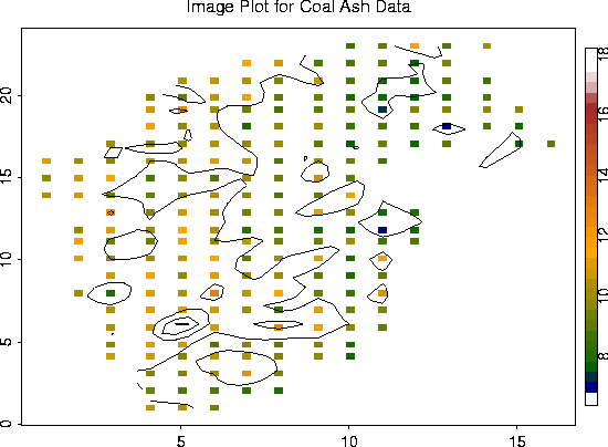
Data obtained from Gomez and Hazen (1970, Tables 19 and 20) on coal ash for the Robena Mine Property in Greene County Pennsylvania.

Overall plot of the data.

# -- Create an image plot of the data. For fun, add the contour lines.
look <- as.image( coalash$y, x=coalash$x)
image.plot( look)
contour( look, add=T, labex=0)

# -- Perform a Krig fit using exponential covariance function with range
# -- paramter, theta=2.5 (choice of theta will be explained below).

fit <- Krig( coalash$x, coalash$y, cov.function = exp.cov.S, theta=2.5)
summary( fit)

Call:

Krig(x = coalash$x, Y = coalash$y, cov.function = exp.cov.S)



Number of Observations:                        208   
Number of unique points:                       208   
Degree of polynomial null space ( base model): 1     
Number of parameters in the null space         3     
Effective degrees of freedom:                  29.7  
Residual degrees of freedom:                   178.3 
MLE sigma                                      1.02  
GCV est. sigma                                 1.018 
MLE rho                                        0.2829
Scale used for covariance (rho)                0.2829
Scale used for nugget (sigma^2)                1.04  
lambda (sigma2/rho)                            3.675 

RESIDUAL SUMMARY:
    min   1st Q   median  3rd Q   max 
 -2.169 -0.6578 -0.09917 0.4115 6.169

COVARIANCE MODEL: exp.cov.S

DETAILS ON SMOOTHING PARAMETER:
 Method used:   GCV    Cost:  1
 lambda   trA   GCV GCV.one GCV.model  shat 
  3.675 29.69 1.209   1.209        NA 1.018

 Summary of estimates for lambda
        lambda   trA   GCV  shat 
    GCV  3.675 29.69 1.209 1.018
GCV.one  3.675 29.69 1.209 1.018

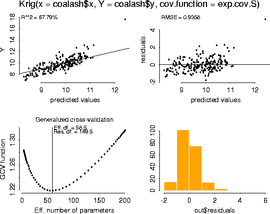
plot( fit)

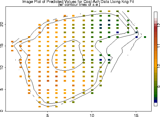
# -- We will use the S-Plus generic function, predict, to make predictions,
# -- using the Krig object fit.
# -- We also added the contours of the standard errors of the estimates.
fit.pred <- predict( fit)
look <- as.image( fit.pred, x=coalash$x)
image.plot( look)

fit.se <- predict.se( fit)
look2 <- as.image (fit.se, x=coalash$x)
contour( look2, add=T, labex=0)

In the above fit, we used the range parameter, theta=2.5. This range parameter was chosen by re-doing the above steps with varying theta parameters and choosing the value that yielded the smallest GCV minimum. The following table shows the GCV minimum results of using various values for theta. From this table, it appears that after theta = 2.5, the GCV minimum does not get much smaller, and so there is little improvement in the average prediction error. Another approach to determne the range parameter is discussed below.

theta	GCV Minimum
0.5 0.75 1.0 1.25 1.5 1.75 2.0 2.25 2.5 2.75 3.0 3.25 3.5 3.75 4.0 4.25 5.0 10.0 100.0	1.225 1.221 1.218 1.216 1.214 1.212 1.211 1.21 1.209 1.209 1.208 1.208 1.207 1.207 1.207 1.207 1.206 1.205 1.205

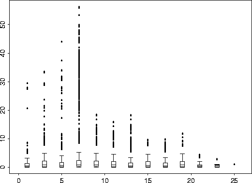
Finding an appropriate covariance function can be a difficult modeling exercise by itself. However, to estimate the parameters of a covariance function, it is possible to utilize well-established methodologies. One straightforward approach is to use nonlinear least squares fitting of the variogram. Fields has a variogram function, viz. vgram.

coalash.vgram <- vgram( coalash$x, coalash$y)

# -- coalash.vgram is a list object. Where "d" are the distances,
# -- coalash.vgram$vgram is the variogram, and call tells how the vgram function was called.
names( coalash.vgram)
[1] "d" "vgram" "call"

Now it is possible to plot the variogram against the distances to get a feel for the type of covariance function, and for the parameters. To do this, we make use of another Fields function. Namely, bplot.xy. This function simply bins y values according to their x values and produces a boxplot of these groups from binning.

bplot.xy( coalash.vgram$d, coalash.vgram$vgram)

Plot from above command.

Same plot, but zoomed in ( ylim=c(0, 10) ).

Indeed, the plots might suggest an alternative covariance matrix to the exponential. Never-the-less, for the purpose of demonstrating the software, we will use the exponential covariance function.

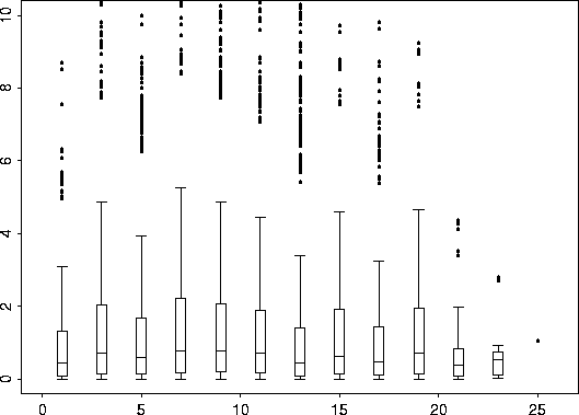Now we use the S-Plus function, nls (Non Linear Least Squares Regression) to search for a suitable range parameter. Simultaneously, we search for possible values for sigma2 and rho which we can subsequently fix, if desired, for the Krig fit. vgram.fit <- nls( vgram ~ sigma2*(1-rho*exp(-d/theta)), coalash.vgram, start=list( sigma2= 9, rho=0.95, theta=1)) summary( vgram.fit)

Formula: vgram ~ sigma2 * (1 - rho * exp( - d/theta))

Parameters:
          Value Std. Error  t value 
sigma2 1.696190  0.0334569 50.69770
   rho 0.750553  0.2807990  2.67292
 theta 1.635050  0.5580010  2.93019

Residual standard error: 3.60828 on 21523 degrees of freedom

Correlation of Parameter Estimates:
      sigma2    rho 
  rho -0.346       
theta  0.566 -0.877

These results suggest theta = 1.63505, and we can also try fixing sigma2 = 1.696190 and rho = 0.750553.

fit <- Krig( coalash$x, coalash$y, theta=1.635050, sigma2=1.696190, rho=0.750553)
summary( fit)


CALL:
Krig(x = coalash$x, Y = coalash$y, rho = 0.750553, sigma2 = 1.69619, theta = 
        1.63505)
                                                       
 Number of Observations:                        208   
 Number of unique points:                       208   
 Degree of polynomial null space ( base model): 1     
 Number of parameters in the null space         3     
 Effective degrees of freedom:                  48.8  
 Residual degrees of freedom:                   159.2 
 MLE sigma                                      0.9604
 GCV est. sigma                                 0.9647
 MLE rho                                        0.4082
 Scale used for covariance (rho)                0.7506
 Scale used for nugget (sigma^2)                1.696 
 lambda (sigma2/rho)                            2.26  

RESIDUAL SUMMARY:
    min   1st Q  median  3rd Q   max 
 -1.899 -0.5541 -0.1009 0.3808 5.486

COVARIANCE MODEL: exp.cov

DETAILS ON SMOOTHING PARAMETER:
 Method used:   user    Cost:  1
 lambda  trA   GCV GCV.one GCV.model   shat 
   2.26 48.8 1.216   1.216        NA 0.9647

 Summary of estimates for lambda
        lambda   trA   GCV   shat 
    GCV  3.422 37.27 1.213 0.9979
GCV.one  3.422 37.27 1.213 0.9979

From this we see that the MLE sigma has been reduced to 0.9064 from 1.02. The GCV minimum is a little higher, and the effective degrees of freedom has been increased to 48.8 from 29.7 when we used GCV to find sigma2, rho, and subsequently lambda.

This is software for statistical research and not for commercial uses. The authors do not guarantee the correctness of any function or program in this package. Any changes to the software should not be made without the authors permission.

Last modified: Dec 21 2005 by thoar@ucar.edu