|
Table of Contents |
|
1. Introduction
2. Thin Plate Splines: Tps 3. Spatial Process Models: Krig 4. Simulating Random Fields (sim.rf) 5. Spatial Predictions for Large Data Sets
|
|
Printable version of Fields Manual
Back to Fields Home Page |
Ozone Concentrations in Chicago
Although not a very interesting data set, it is useful for demonstrating the Krig package.
Overall plots of the data:
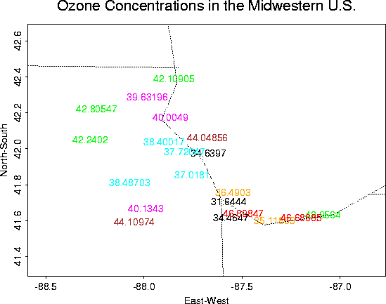 Close-up |
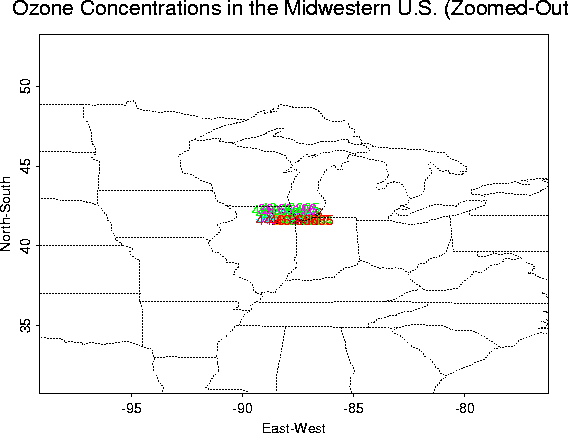 Zoomed-out (to see location better) |
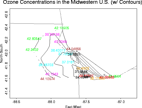 Contour Plot |
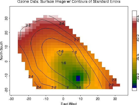
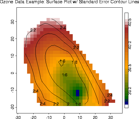 Surface Plot w/ Standard Errors from Krig fit |
# -- Find the Krig fit to the ozone data using
# -- Exponential covariance function. Choice of range parameter, theta, is
# -- arbitrarily chosen here to be 10 miles.
fit <- Krig(ozone$x, ozone$y, exp.cov, theta=10)
# -- Print summary of the Krig fit.
# -- The summary function is a generic S-Plus function that is used to provide
# -- summary information about a regression object. For example, from the
# -- output of the summary below, we can discern that 4 or 5 parameters
# -- (Effective df=4.5) are needed to fit the model. Also, the estimate for
# -- sigma is about 4.2 (both MLE and GCV give this), and for rho is 2.374.
summary( fit)
Call:
Krig(x = ozone$x, Y = ozone$y, cov.function = exp.cov, theta = 10)


Number of Observations:				20
Number of unique points:			20
Degree of polynomial null space ( base model):  1
Number of parameters in the null space		3
Effective degrees of freedom:			4.5
Residual degrees of freedom:			15.5
MLE sigma					4.206
GCV est. sigma					4.2
MLE rho						2.374
Scale used for covariance (rho)			2.374
Scale used for nugget (sigma^2)			17.69
lambda (sigma2/rho)				7.453
Cost in GCV					1
GCV Minimum					22.8

 Residuals:
    min  1st Q  median 3rd Q   max
 -7.037 -2.189 -0.4681 2.299 7.382
 REMARKS
Covariance function: exp.cov
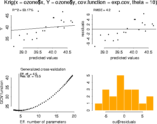
# -- Obtain diagnostic plots of the fit using the generic function, plot.
# -- This is the same function used for other standard S-Plus regression
# -- objects. Note that the plots of the residuals suggest that the model is
# -- overfitting ozone at lower values.
plot( fit)
# -- Calculate the standard errors of the Krig fit using the Fields function
# -- predict.se.Krig, which finds the standard errors of prediction based on a linear
# -- combination of the observed data--generally the BLUE. The only required
# -- argument is the Krig object itself. Optional arguments include alternate
# -- points to compute the standard error on, viz. x, a covariance function, rho, sigma2
# -- (default is to use the values passed into Krig originally),
# -- and some other logical parameters that can be found in the help file.
ozone.fit.se <- predict.se( fit)
out.p <- predict.surface( fit)
image.plot( out.p, xlab="East-West", ylab="North-South")
out2.p <- predict.surface.se( fit)
contour( out2.p, add=T)
# -- It is also possible to obtain krig predictions at other locations besides
# -- those given with the data. For example,
# -- Here, I choose a random set of points to predict at. I did this to
# -- emphasize that you can choose any grid points that you want
# -- to study.
loc.knot <- cbind (runif( 20, min=-30, max=35), runif( 20, min=21, max=36))
# -- Now predict with these points.
ozone.pred2 <- predict( fit, loc.knots)
# -- We can also use predict to obtain predictions for the ozone fit using a
# -- different value for lambda, or df--and, indeed, different data.
# -- For example,
ozone.pred3 <- predict( fit, lambda=5)