[an error occurred while processing this directive]
Fields: Web Manual
Table of Contents
1. Introduction

2. Thin Plate Splines: Tps 3. Spatial Process Models: Krig 4. Simulating Random Fields (sim.rf)

5. Spatial Predictions for Large Data Sets
6. Other Fields Functions References

Printable version of Fields Manual

Back to Fields Home Page
Daily 8-Hour Ozone Data Example
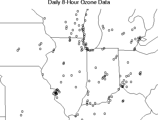
The Fields dataset ozone2 consists of daily 8-hour surface ozone measurements during the summer of 1987 for approx. 150 locations in the Midwest.


# Plot the data with a map of the area.
usa( xlim= range( ozone2$lon.lat[,1]), ylim= range( ozone2$lon.lat[,2]))
points( ozone2$lon.lat, pch="o")
title("Daily 8-Hour Ozone Data", cex=0.85)

Veiw Full Size Plot

For daily ozone measurements it has been found that a non-stationary covariance with an isotropic correlation function is a useful model. Let x be a vector of locations, Y(x) the ozone measurement at location x, and obtain the standardized process

Z(x) = ( Y(x) - EY(x) ) / sqrt(Var( Y(x) ))


We will assume that this new process is isotropic, and assuming that the spatial fields EY(x) and Var( Y(x) ) are known, it is easy to use Krig to obtain spatial estimates, incorporating this more complex covariance.

It will be handy to create a correlogram before we continue.

ozone.cor <- COR( ozone2$y)

The Fields function COR is useful because it will omit missing values in computing pairwise correlations and also contains marginal means and standard deviations. Next, we will use this correlation object to estimate the marginal mean, EY(x), and standard deviation, sqrt( Var( Y(x) )) surfaces using the different days as replicates. The use of return.matrices = F is optional and simply reduces the size of the returned object. This way, the large matrices used in finding the standard errors will not be included in the returned object.

mean.tps <- Tps( ozone2$lon.lat, ozone.cor$mean, return.matrices = F)
sd.tps <- Tps( ozone2$lon.lat, ozone.cor$sd, return.matrices = F)


Now we are ready to fit the Krig model to this data, Krig does not accept missing values, so we need to remove them in some fashion before calling Krig. For this example, we will fit the model for day 16. Notice the use of: cov.function=exp.earth.cov, sd.obj=sd.tps, mean.obj=mean.tps, and m=1. exp.earth.cov is an exponential covariance function that uses great circle distances for locations reported in longitude and latitude. The Tps objects are used to define the mean and standard deviation fields for standardizing the measurements. They are estimates of the marginal mean and standard deviation surfaces which we use to take into account the lack of stationarity in the data set. Since we are including a mean field, it is appropriate to fit a constant term for the polynomial part of the model, thus we include the option, m = 1. Finally, we use a range parameter estimated from nonlinear least squares fitting of the correlogram. An example of this procedure appears in the previous coal ash example.

day16 <- c( ozone2$y[16,])

# -- Logical vector to remove missing values from day16.
idn <- !is.na( day16)
fit <- Krig( ozone2$lon.lat[idn, ], day16[idn], cov.function=exp.earth.cov, theta = 343, sd.obj=sd.tps, mean.obj=mean.tps, m=1) summary( fit)

Krig(x = ozone2$lon.lat[idn,  ], Y = day16[idn], cov.function = exp.earth.cov,
        m = 1, mean.obj = mean.tps, sd.obj = sd.tps, theta = 343)
                                                        
 Number of Observations:                        147    
 Number of unique points:                       147    
 Degree of polynomial null space ( base model): 0      
 Number of parameters in the null space         1      
 Effective degrees of freedom:                  114.7  
 Residual degrees of freedom:                   32.3   
 MLE sigma                                      0.289  
 GCV est. sigma                                 0.3172 
 MLE rho                                        7.538  
 Scale used for covariance (rho)                7.538  
 Scale used for nugget (sigma^2)                0.0835 
 lambda (sigma2/rho)                            0.01108
 Cost in GCV                                    1      
 GCV Minimum                                    0.4585 

Y is standardized before spatial estimate is found
 Residuals: 
     min    1st Q   median   3rd Q   max 
 -0.6091 -0.07774 0.003612 0.08233 0.433
 REMARKS
Covariance function: exp.earth.cov 
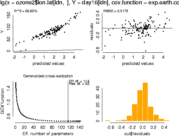

From the above summary, we can see that there are 147 observations, all of which are unique. A constant term was used for the polynomial part of the model--as we specified with m = 1. The large effective degrees of freedom in the model (114.7) found by GCV will result in a surface that fits the observations closely. Note that the GCV function (left lower graph) is fairly flat from 30 d.f. and suggests that the value of lambda can not be well estimated from in sample average prediction error.

View Full Size Plot


This is software for statistical research and not for commercial uses. The authors do not guarantee the correctness of any function or program in this package. Any changes to the software should not be made without the authors permission.

Last modified: Dec 21 2005   by thoar@ucar.edu